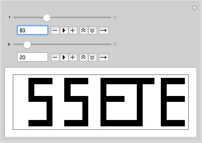
Here's a rather fun snippet of code from my increasingly large notebook of interesting CA programs:
init=
{{1,1,1,1,1,0,1,1,1,1,0,0,1,1,1,1,0,0,1,1,1,1,0,0,1,1,1,1},
{0,0,1,0,0,0,1,0,0,0,0,0,1,0,0,0,0,0,1,0,0,0,0,0,1,0,0,0},
{0,0,1,0,0,0,1,0,0,0,0,0,1,0,0,0,0,0,1,0,0,0,0,0,1,0,0,0},
{0,0,1,0,0,0,1,1,1,1,0,0,1,1,1,1,0,0,1,1,1,1,0,0,1,1,1,1},
{0,0,1,0,0,0,1,0,0,0,0,0,0,0,0,1,0,0,0,0,0,1,0,0,1,0,0,0},
{0,0,1,0,0,0,1,0,0,0,0,0,0,0,0,1,0,0,0,0,0,1,0,0,1,0,0,0},
{0,0,1,0,0,0,1,0,0,0,0,0,0,0,0,1,0,0,0,0,0,1,0,0,1,0,0,0},
{1,1,1,0,0,0,1,1,1,1,0,0,1,1,1,1,0,0,1,1,1,1,0,0,1,1,1,1}};

tostep[r_,s_,init_]:=Table[CellularAutomaton[r,i,{{s}}][[1]],{i,init}]
<!-- this is to separate the two code blocks. it's a useful trick! -->
ArrayPlot[init]

ArrayPlot[tostep[30, 20,init]]

Manipulate[
 ArrayPlot[tostep[r, s,init]], {{r, 30}, 1, 255, 1}, {{s, 20}, 0, 200, 1}]

It's interesting to see what rule and step combinations result in a resemblance to the original matrix.