Message Boards Message Boards

1
|
17508 Views
|
6 Replies
|
1 Total Likes
View groups...
Share
Share this post:

Different bode plots for the same input in mathematica, wolfram alpha

Posted 10 years ago

The phase diagrams of both look wrong to me. What am I missing?

Wolframalpha Mathematica

POSTED BY: riccardo loddo
6 Replies
Posted 10 years ago

Hi Jos,

I don't get an error when I evaluate your notebook. Perhaps some variable is defined. I suggest starting with a fresh kernel.

Best, David

In[6]:= sysOutput = 
 OutputResponse[sys, UnitStep[t], t] // Chop  (* ERROR ?? *)

Out[6]= {2. (-1. Cos[0.707107 t] UnitStep[t] + 
    1. Cos[0.707107 t]^2 UnitStep[t] + 
    0.000707107 Sin[0.707107 t] UnitStep[t] + 
    1. Sin[0.707107 t]^2 UnitStep[t])}
POSTED BY: David Keith

Hi David,

Thanks, all works fine..................Jos

POSTED BY: Jos Klaps

Hi David,

I got an error from sysOutput line and I don't know why? See file attached.

Can you help.....Thanks

Attachments:
POSTED BY: Jos Klaps
Posted 10 years ago

You can get, what I think you are looking for, by doing the following.

BodePlot[tf, PlotLayout -> "Phase", PhaseRange -> {-\[Pi], \[Pi]}]

enter image description here

In v10, an unnecessary (but mathematically not incorrect) phase lag of 360 gets added.

POSTED BY: Suba Thomas
Posted 10 years ago

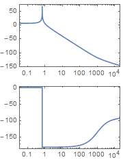
I would also be grateful for responses to this from those with experience using Mathematica for control theory. In the code below, I treat the transfer function as that of the complete system. (Not a component with feedback around it.)

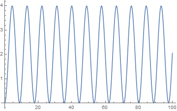
I observe that the transfer function is unstable, with conjugate poles on the axis. The OutputResponse to a step is oscillatory. I don't think a Bode plot of such a system is meaningful.

syss = (1 + 0.001 s)/(s^2 + 0.5);

sys = TransferFunctionModel[{{syss}}, s];

BodePlot[sys, FeedbackType -> None, PhaseRange -> {-Pi, Pi}]
enter image description here

In[4]:= (* poles on the axis == unstable *)
TransferFunctionPoles[sys]

Out[4]= {{{0. - 0.707107 I, 0. + 0.707107 I}}}

In[5]:= sysOutput = OutputResponse[sys, UnitStep[t], t] // Chop

Out[5]= {2. (-1. Cos[0.707107 t] UnitStep[t] + 
    1. Cos[0.707107 t]^2 UnitStep[t] + 
    0.000707107 Sin[0.707107 t] UnitStep[t] + 
    1. Sin[0.707107 t]^2 UnitStep[t])}

In[6]:= Plot[sysOutput, {t, 0, 100}]
enter image description here

POSTED BY: David Keith

Thank you, we will look into this.

POSTED BY: EDITORIAL BOARD
Reply to this discussion
Community posts can be styled and formatted using the Markdown syntax.
Reply Preview
Attachments
Remove
or Discard

Group Abstract Group Abstract