Unless you use EXACTLY the syntax and capitalization shown in the help pages then Mathematica will not understand and will give you error messages or incorrect results or even nothing at all

Mathematica has no "sense." If someone were to write a sentence in English or Italian for you and they were to incorrectly fail to capitalize a name or make a small error in grammar then you would likely understand some or most of what they wrote. If you write a sentence for Mathematica and fail to correctly capitalize a name or make a small error in grammar then Mathematica has absolutely no idea what you mean.

plot[function[...]] means absolutely nothing to Mathematica and it returns the input unchanged.

In[1]:= plot[AppellF1[1/2, 1, 1, 3, -1, -2]]

Out[1]= plot[AppellF1[1/2, 1, 1, 3, -1, -2]]

Plot[function[...]] means absolutely nothing to Mathematica and it returns an error message and the input unchanged.

In[2]:= Plot[AppellF1[1/2, 1, 1, 3, -1, -2]]

During evaluation of In[2]:= Plot::argr: Plot called with 1 argument; 2 arguments are expected. >>

Out[2]= Plot[AppellF1[1/2, 1, 1, 3, -1, -2]]

Plot[function[...],{variable, minvalue,maxvalue}] Mathematica understands, but this may take hours or days or months to calculate hundreds or thousands of points.

In[3]:= Plot[AppellF1[1/2, 1, 1, 3, (1/(1 - \[Gamma]/2)), (1/(1 - 3 \[Gamma]/4))], {\[Gamma], 0, 15}]

Out[3]= $Aborted

Now

This works

In[4]:= AppellF1[1/2, 1, 1, 3, -1, -1]

Out[4]= -(4/3) (-2 + Sqrt[2])

This Mathematica cannot find an exact numeric value for and so returns the original expression

In[5]:= AppellF1[1/2, 1, 1, 3, -1, -3]

Out[5]= AppellF1[1/2, 1, 1, 3, -1, -3]

This works

In[6]:= Table[AppellF1[1/2, 1, 1, 3, -1, x], {x, -1, 1}]

Out[6]= {-(4/3) (-2 + Sqrt[2]), 4/3 (-5 + 4 Sqrt[2]), 8/3 (-1 + Sqrt[2])}

This works for some points and there is no exact solution for other points

In[7]:= Table[AppellF1[1/2, 1, 1, 3, -1, x], {x, -2, 5}]

Out[7]= {AppellF1[1/2, 1, 1, 3, -1, -2],
 -(4/3) (-2 + Sqrt[2]), 4/3 (-5 + 4 Sqrt[2]), 8/3 (-1 + Sqrt[2]),
 AppellF1[1/2, 1, 1, 3, -1, 2], AppellF1[1/2, 1, 1, 3, -1, 3], AppellF1[1/2, 1, 1, 3, -1, 4], AppellF1[1/2, 1, 1, 3, -1, 5]}

This works and there are approximate solutions, real and complex, for each point

In[8]:= Table[N[AppellF1[1/2, 1, 1, 3, -1, x]], {x, -2, 5}]

Out[8]= {0.719064,
 0.781049, 0.875806, 1.10457, 
 1.1808241108855023 - 0.4444444444444443 I, 0.996729 + 0.628539 I, 0.841828 + 0.69282 I, 0.723745 + 0.711111 I}

This finds the real approximate component for the points

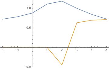
In[9]:= repoints = Table[{x, Re[N[AppellF1[1/2, 1, 1, 3, -1, x]]]}, {x, -2, 5}]

Out[9]= {{-2, 0.719064}, {-1, 0.781049}, {0, 0.875806}, {1, 1.10457},
 {2, 1.1808241108855023}, {3, 0.996729}, {4, 0.841828}, {5, 0.723745}}

This finds the complex approximate component for the points

In[10]:= impoints = Table[{x, Im[N[AppellF1[1/2, 1, 1, 3, -1, x]]]}, {x, -2, 5}]

Out[10]= {{-2, 0}, {-1, 0}, {0, 0}, {1, 0},
 {2, -0.4444444444444443}, {3, 0.628539}, {4, 0.69282}, {5, 0.711111}}

This overlays two plots, the approximate real and complex magnitudes for each point and joins them with lines

In[11]:= g1 = ListPlot[{repoints, impoints}, Joined -> True, PlotRange -> {-.5, 1.2}];

If you can more precisely describe exactly what points you wish to plot then it may be possible to show how to do that in reasonable time but, as you can easily verify for yourself, for many values of x the calculation time for your function is very very long.