Well

In[33]:= Clear[e, k, \[HBar], c, \[Omega], T, \[Tau], \[Sigma]]
e = Quantity["ElementaryCharge"];
k = Quantity["BoltzmannConstant"];
\[HBar] = Quantity["ReducedPlanckConstant"];
c = Quantity["SpeedOfLight"];
(* \[Omega]=2 \[Pi] c/\[Lambda];
\[Lambda] = Quantity[445,"Nanometers"]; 
\[Tau] =Quantity[0.2,"Picoseconds"]; *)
T = Quantity[300, "Kelvin"];
\[Sigma][\[Mu]_, \[Omega]_, \[Tau]_] := 
 I (e^2 k T)/(\[Pi] \[HBar]^2 (\[Omega] + I/\[Tau])) (\[Mu]/(k T) + 
     2 Log[Exp[-\[Mu]/(k T)] + 1]) + 
  I e^2/(4 \[Pi] \[HBar]) Log[(2 Abs[\[Mu]] - \[HBar] (\[Omega] + 
          I/\[Tau]))/(2 Abs[\[Mu]] + \[HBar] (\[Omega] + I/\[Tau]))]

In[40]:= \[Sigma][Quantity[0.2, "ElectronVolts"], 
 2 \[Pi] c/Quantity[1400, "Nanometers"], Quantity[0.2, "Picoseconds"]]

Out[40]= Quantity[(1.90904  - 0.0426355 I), (
 "BoltzmannConstant" (
  "ElementaryCharge")^2 "Kelvins" \
"Picoseconds")/("ReducedPlanckConstant")^2]

In[41]:= UnitConvert[%]

Out[41]= Quantity[(0.0000608367  - 1.3587*10^-6 I), (("Amperes")^2 (
  "Seconds")^3)/("Kilograms" ("Meters")^2)]

In[46]:= QuantityMagnitude[\[Sigma][Quantity[0.2, "ElectronVolts"], 
  2 \[Pi] c/Quantity[1400, "Nanometers"], 
  Quantity[0.2, "Picoseconds"]]]

Out[46]= 1.90904 - 0.0426355 I

and it is plottable like

  Plot3D[ReIm[QuantityMagnitude[\[Sigma][Quantity[0.4, "Electronvolts"], 
    2 \[Pi] c/Quantity[x, "Nanometers"], 
    Quantity[y, "Picoseconds"]]]], {x, 1400, 1600}, {y, 0.1, 0.5}, PlotPoints -> 10, MaxRecursion -> 0]

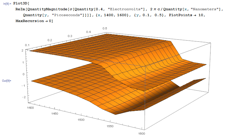
The real part is above. If one unuses the options PlotPoints -> 10, MaxIterations -> 0 the plot takes a very long time. Using Quantity in numerics and graphics is definitely an overkill borderlining abuse, the usual method is to compute dimensionless expressions by remembering the actual physical dimension only in plot labels and axes labels.

Some more considerations are necessary: If $\omega$ has the dimension of an inverse length and $\tau$ has dimension of inverse time (Hertz), then the sum $\omega + \frac{i}{\tau}$ has incompatible units. With other words, if the chemical potenial $\mu$ has unit Gibbs then the sum $\omega + \frac{i}{\tau}$ needs dimension

In[121]:= UnitConvert["Gibbs"/"ReducedPlanckConstant"]
Out[121]= Quantity[9.482522*10^33, 1/("Moles" "Seconds")]

with other words Hertz/Moles. Let's say you fix that, you can in principle go ahead as follows

Clear[e, k, \[HBar], c, \[Omega], T, \[Tau], \[Sigma]]
e = Quantity["ElementaryCharge"];
k = Quantity["BoltzmannConstant"];
\[HBar] = Quantity["ReducedPlanckConstant"];
c = Quantity["SpeedOfLight"];
(* \[Omega]=2 \[Pi]/\[Lambda];
\[Lambda] = Quantity[445,"Nanometers"]; *)
\[Tau] = Quantity[2178, "Hertz"];
T = Quantity[300, "Kelvin"];
\[Sigma][\[Mu]_, \[Omega]_] := 
 I (e^2 k T)/(\[Pi] \[HBar] (\[Omega] + I/\[Tau])) (\[Mu]/(k T) + 
     2 Log[Exp[-\[Mu]/(k T)] + 1]) + 
  I e^2/(4 \[Pi] \[HBar]) Log[(2 Abs[\[Mu]] - \[HBar] (\[Omega] + 
          I/\[Tau]))/(2 Abs[\[Mu]] + \[HBar] (\[Omega] + I/\[Tau]))]

calling it like

\[Sigma][Quantity[1.4, "Gibbs"], 2 \[Pi]/Quantity[445, "Nanometers"]]

to get an error message

Quantity::compat: 1/(Nanometers) and 1/(Hertz) are incompatible units >>

of course.