Try breaking the problem up into simpler things.
(1) You need the correct syntax for a Mathematica function:
w[x_,y_] := Cos[x] Sin[y]
[I'm presuming that your ambiguous expression cosx.siny means, in traditional math notation, (cos x) (sin y) rather than cos(x sin y).]
(2) Then a 3d plot would be given by:
Plot3D[w[x, y], {x, -3 Pi/2, 3 Pi/2}, {y, -3 Pi/2, 3 Pi/2}]
(3) Add one specific y = constant, say y = 2.25, slice by using a corresponding value for option Mesh:
yTrace = Plot3D[w[x, y], {x, -3 Pi/2, 3 Pi/2}, {y, -3 Pi/2, 3 Pi/2},
   Mesh -> {{-5}, {{2.25, Directive[Thick, Red]}}},
   PlotStyle -> LightBlue, AxesLabel -> {x, y, z}]
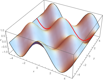
(The first entry {-5} in the value of Mesh is a "dummy" value for an x-slice, chosen to be outside the specified x-domain.)
(4) Do a similar thing for one specific x = constant slice.
(5) Construct a Manipulate in a simple form just for varying the constant in, say, y = constant.
(6) Repeat (5) for x = constant.
(7) Put the results of (5) and (6) together.
Note: You'll find this sort of thing already created in the Wolfram Demonstration:
http://demonstrations.wolfram.com/CrossSectionsOfGraphsOfFunctionsOfTwoVariables/
(I found that Demonstration simply by Googling "mathematica slice 3d plot".)
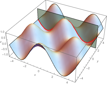
If you want to show the plane y = constant that makes the slice, combine the Plot3D with an appropriate ContourPlot3D:
 ySlice = ContourPlot3D[y == 2.25, {x, -3 Pi/2, 3 Pi/2}, {y, -3 Pi/2, 3 Pi/2}, {z, -1, 1},
                   ContourStyle -> Opacity[0.5, Lighter@Green], Mesh -> None]
Then combine yTrace with ySlice using Show:
Show[{yTrace, ySlice}]
Note that I made no serious attempt to make the 3d graphics look as clear and appealing as possible. Doing such things takes a lot of work (at least for me).


