Message Boards Message Boards

0
|
10217 Views
|
9 Replies
|
4 Total Likes
View groups...
Share
Share this post:

Simple way to plot functions & vector properties

Posted 9 years ago

I'm trying to get a better intuition for scalar and vector fields, so thought I'd experiment with Plot3D .. For example I wanted to plot a function like x^2 + xy + y^2, easy enough. Then I wanted to see what the gradient looked like - could only find an abstruse set of nested commands. I will also want to look at divergence and curl, so combinations of scalars and vectors plus these operators ....

Is there a simple and easy to remember way to do things like this? Thanks.

POSTED BY: Alan Smith
9 Replies
Posted 9 years ago

the Wolfram Demonstrations Project has a number of useful bits for gradient, but nothing along those lines for divergence and curl - so maybe someone will see this and build some demonstrations for those as well :-) $X^2 + x*y + y^2$ is just an example off the top of my head, another I liked was at https://www.wolfram.com/mathematica/new-in-8/new-and-improved-scientific-and-information-visualization/show-the-gradient-field-on-a-surface.html and of course some trig combination functions ....anyway, thanks for your interest & time David

POSTED BY: Alan Smith
Posted 9 years ago

Thanks David, while you make a great deal of sense, I am writing an exam in the not-too-distant and for now my goal is just to plot a few simple 3-D functions with their associated grad/div/curl - to help me visualise them and the differences between them; I don't know mathematica at all well and don't want to get side-tracked (now) in trying to learn it well enough.

My thought was that I could find examples of each of any simple function with it's grad/div/curl and could code them in a macro - I could get a lot of visualising done quite time-cheaply. Do you (or anyone) perhaps know of a simple example of 'recording a macro' I could look at?

POSTED BY: Alan Smith

You can find some examples and pictures of these items in Wikipedia or perhaps other places on the web. You could look up Grad, Div, Curl, VectorPlot, VectorPlot3D, ContourPlot and ContourPlot3D in Mathematica Documentation but you will probably not be able to put them together in a short time. You might look in the Wolfram Demonstrations Project for examples. Unfortunately, Mathematica is not quite an off-the-self and start using application and I don't know of an existing direct application that would help you.

In regard to building a MyGradPlot function: Yes you could do that but I would recommend against starting out on that path, although you might eventually come back to it. The reason is that presenting information in a graphical form is as much an art as it is a science. (I recommend the books by Edward Tufte on data visualization for a taste of this.)

How you present graphical information depends strongly on the information you're presenting, in this case functions and their gradients. There are an awful lot of just 2-dimensional functions. How many have you presented in a graphical manner, with their gradients, so far? May I guess that it's not even one? And how many do you wish to make in the near future? Enough to spend the time to write a fairly general MyGradPlot?

Some functions might have a small range of values and only slowly changing gradient fields. Some may have wildly changing gradient fields, twisting and turning with large and small amplitudes. Some functions might have large nearly level plateaus and other regions with rapid variation. Would your routine be adaptive enough to give good representations of all of these?

Then there are many different techniques that could be used to present the information.

1) A dynamic Locator on a contour plot with a vector giving the gradient. Or a unit vector giving the gradient direction and a tooltip or label giving the amplitude.

1a) A dynamic Locator plot with the addition of a panel giving textual and numerical information: coordinates of the locator, value of the function, vector value of the gradient. Combining graphical and textual-numerical information in one dynamic display is a very powerful technique.

2) A contour plot with a grid of vectors giving the gradient. But this is poor with a wide range of gradient values or rapid change in a small region. Too many vectors just give you a confused or black screen.

3) A 3D plot of the surface with the gradient amplitude color coded on the surface.

4) An overall plot of the function and gradient and close-up plots of critical regions.

I'm sure there are many other techniques that could be used.

If your object is just to learn some math and physics and Mathematica usage, I would recommend doing some plots with varying functions as individual graphics, and dynamics if possible. You will learn more, and faster, about functions, gradients and Mathematica and have more fun, then undertaking a rather arduous task.

Of course, there might be cases where you are dealing with only a limited range of functions and you could easily write a function where all one had to do is plug in the function. The right hand side of your definition would probably be a Module where you calculated the various parts of the graphics and then assembled them for display. Even here, if you had a wider range of experience with the various methods and techniques, this would be much easier.

Posted 9 years ago

Hi folks, lost my PC to the Win10 upgrade (it got into an endless auto-repair loop and I eventually had to rebuild, so be warned) - and waiting for Wolfram support so I can reinstall mathematica ....

In the meantime I wondered - is there a way to build a 'macro' in mathematica, so I could (for example) build 'MyGradPlot[function, range(s)] and just vary the functions? If there is, I learn best by looking at examples :-)

Thanks

POSTED BY: Alan Smith

The following is a rather extended solution using two packages I'm involved with. The GrassmannCalculus package, which I am developing with John Browne. It is rather extensive and you can get information about it here:

GrassmannCalculus

The Presentations package, which I sell, has I think a more convenient graphics paradigm dealing directly in terms of graphics primitives. In any case, you could stay with the Mathematica Grad function and the Show statement for combining graphics.

<< GrassmannCalculus`
<< Presentations`

We set a 2-dimensional vector space using orthonormal basis vectors.

SetEuclideanNSpace[2, {x, y}, "Orthonormal"]

Here is your function:

f[x_, y_] := x^2 + x y + y^2 

The gradient can be calculated very simply with Mathematica.

Grad[f[x, y], {x, y}]

giving

{2 x + y, x + 2 y}

It can also be calculated in GrassmannCalculus, in which case we obtain a vector expression in terms of the orthonormal vectors. In Grassmann algebra the vectors are always maintained and are not only part of the notation but also elements of the algebra.

step1 = GrassmannGrad[f[x, y]]

giving

enter image description here

The following expression converts it to the component list as with Mathematica.

step1 // ToListCoordinates

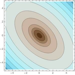
We draw the contour plot. ContourDraw is basically like ContourPlot but extracts the primitives. Except here I'm using an extra feature of Presentations called ContourColors. It adjusts the colors between contours so that each region has a distinct color or shading even if some contours are close together in value and others far apart.

functionDraw =
  Module[{contourList},
   contourList = Union[{0, 0.1, 0.5, 1, 2, 5}, Range[10, 80, 10]];
   ContourDraw[f[x, y], {x, -5, 5}, {y, -5, 5},
    Contours -> contourList,
    ColorFunctionScaling -> False,
    ColorFunction -> 
     ContourColors[contourList, ColorData["BrownCyanTones"]]]
   ];

This plots the function. In the notebook the contour values will be labeled with tooltips.

Draw2D[
 {functionDraw},
 Frame -> True,
 ImageSize -> 300]

enter image description here

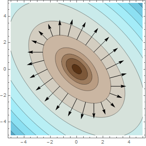
Now the question is how to draw the gradient vectors? Often we might fill the entire plot with vectors, but this often gets cluttered. I like to minimize the number of vectors. Sometimes it's useful to just have a single vector attached to a Locator that you can drag around the plot and explore the gradient. I'm going to put a single set of gradient vectors around one of the contours. This won't clutter the plot too much and the pattern is similar for all contours.

For this we need to find a parametrization for the ellipse. This involved most of the work. The standard ellipse is parametrized by:

ellipse1[a_, b_][t_] := {a Cos[t], b Sin[t]}

You can check that this parametrizes:

p^2/a^2 + q^2/b^2 == 1;

It's clear that the contour ellipses are rotated by 45 degrees. We'll need a rotation matrix and rules for transitioning between x,y and p,q coordinates.

rotationMatrix[t_] = {{Cos[t], -Sin[t]}, {Sin[t], Cos[t]}};
pqRotationRules[t_] = Thread[{p, q} -> rotationMatrix[t].{x, y}];
xyRotationRules[t_] = Thread[{x, y} -> rotationMatrix[t].{p, q}]; 

We start with your equation for contour value 5. Rotating it gives the equation in standard form.

x^2 + x y + y^2 == 5
% /. xyRotationRules[\[Pi]/4] // ExpandAll // 
  Collect[#, {x^2, y^2, x y}, Together] &;
Distribute[#/5] & /@ %

giving

x^2 + x y + y^2 == 5
(3 p^2)/10 + q^2/10 == 1

Setting a^2==10/3 and b^2==10, we can write a parametrization for the contour with value 5.

ellipse2[t_] = 
 ellipse1[Sqrt[10/3], Sqrt[10]][t].rotationMatrix[-\[Pi]/4]

giving

{Sqrt[5/3] Cos[t] - Sqrt[5] Sin[t], Sqrt[5/3] Cos[t] + Sqrt[5] Sin[t]} 

Now we need a routine to draw a vector as a function of the angle t.

gradientVectorDraw[t_] :=
 Module[{x, y, grad},
  {x, y} = ellipse2[t];
  grad = {2 x + y, x + 2 y};
  {Arrowheads[0.04], Arrow[{{x, y}, {x, y} + 0.3 grad}]}
  ]

And we can draw the function with a set of gradient vectors.

Draw2D[
 {functionDraw,
  Table[gradientVectorDraw[t], {t, 0, 2 \[Pi] - \[Pi]/12, \[Pi]/12}]},
 Frame -> True,
 ImageSize -> 300]

enter image description here

Posted 9 years ago

Hi - Plot3D will plot the function, but I want to see the gradient (or divergence or curl) simultaneously?

Thanks Alan

POSTED BY: Alan Smith
Posted 9 years ago

Mathematica has an abundance of tools for vector calculus. Some examples are seen in the attached notebook.

Best regards,

David

Attachments:
POSTED BY: David Keith

Hi Alan may be like this Plot3D[(x^2+xy+y^2),{x,1,10},{y,5,17}]

https://reference.wolfram.com/language/ref/VectorPlot3D.html

POSTED BY: Tasneem Smadi
Reply to this discussion
Community posts can be styled and formatted using the Markdown syntax.
Reply Preview
Attachments
Remove
or Discard

Group Abstract Group Abstract