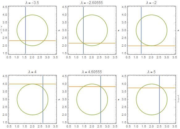
Lagrange multipliers are a common optimization technique which are visualized in a number of different ways. What I show here is a visualization of the equations generated using Lagrange multipliers for finding the points on an off-center circle minimizing and maximizing the distance from the origin. The equation of the circle is circ[{x,y}] == 1 where
circ[{x_, y_}] = (x - 2)^2 + (y - 3)^2 - 1;
The equations can be generated by setting the gradient of the objective function equal to the multiplier times the gradient of the constraint, where the gradient is taken with respect to the problem variables and the multiplier. The gradient with respect to the multiplier reproduces the constraint.
lageqns =
 Thread @ D[x^2 + y^2 == \[Lambda]*circ[{x, y}], {{x, y, \[Lambda]}}]

 {2 x == 2 (-2 + x) \[Lambda], 2 y == 2 (-3 + y) \[Lambda],
 0 == -1 + (-2 + x)^2 + (-3 + y)^2}
Solving the equations gives
NSolve[lageqns]
{{x -> 1.4453, y -> 2.16795, [Lambda] -> -2.60555}, {x -> 2.5547, y -> 3.83205, [Lambda] -> 4.60555}}
The equations can be plotted for various values of the Lagrange multiplier, two of which are values found by solving the equations. For those values, all three curves coincide at the point sought.
Table[ContourPlot[
  Evaluate[lageqns /. \[Lambda] -> \[Lambda]i], {x, .5, 3.5}, {y, 1.5,
    4.5}, PlotLabel ->
   "\[Lambda] = " <>
    ToString[\[Lambda]i]], {\[Lambda]i, {-3.5, -2.60555, -2, 4,
   4.60555, 5}}]