Hi Javid,
OK, here comes annother try: The idea is to use Shannon interpolation, i.e. one obtains a (lengthy) sum of sinc functions as an analytic expression. But to avoid oscillations between data points it is necessary to extend the data in a way so that their values go smoothly towards zero on both sides of the interval. I did this using BSplineFunction. My result finally looks like this (the blue points are your original data, the continuous curve shows the Shannon interpolation):
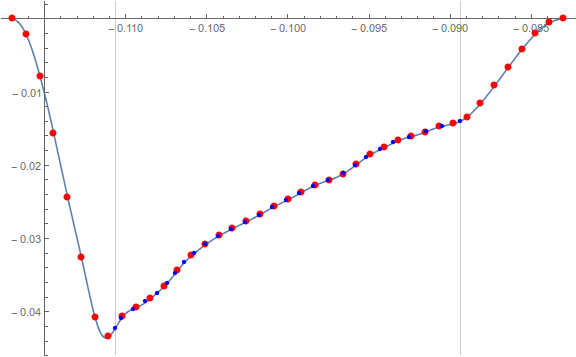
Here is my code; it should be quite self-explaining:
ClearAll["Global`*"]
data  (* = <...your data ...>; *)
data = SortBy[data, First];
{xmin, leftY} = First@data;
{xmax, rightY} = Last@data;
dDelta = (xmax - xmin)/10;
leftF = BSplineFunction[{{xmin, leftY}, {xmin - dDelta,
     leftY - dDelta (rightY - leftY)/(xmax - xmin)}, {xmin - 2 dDelta,
      0}, {xmin - 3 dDelta, 0}}];
rightF = BSplineFunction[{{xmax, rightY}, {xmax + dDelta,
     rightY + dDelta (rightY - leftY)/(xmax - xmin)}, {xmax +
      2 dDelta, 0}, {xmax + 3 dDelta, 0}}];
(* extended data: *)
data1 = SortBy[Join[Table[leftF[t/4], {t, 1, 4}], data, Table[rightF[t/4], {t, 1, 4}]], First];
xmin1 = data1[[1, 1]];
xmax1 = data1[[-1, 1]];
(* aequidistant resampling: *)
dDelta = (xmax1 - xmin1)/40;
ifunc = Interpolation[data1];
idata = Table[{x, ifunc[x]}, {x, xmin1, xmax1, dDelta}];
(* proper definition of sinc function *)
sinc = Sinc[Pi #] &;
(* resulting Shannon interpolation: *)
shannonIP[x_] = Total[#2 sinc[(x - #1)/dDelta] & @@@ idata];
Plot[shannonIP[x], {x, xmin1, xmax1},
 Epilog -> {PointSize[Large], Red, Point[idata], PointSize[Medium],
   Blue, Point[data]}, GridLines -> {{xmin, xmax}, None},
 ImageSize -> Large]
Hope this helps! Regards -- Henrik


