I recently had the pleasure of being accepted into the Wolfram Summer School and decided to conduct a qualitative analysis of the graphical properties of 1D elementary cellular automata to test and improve my WL skills a bit prior to the start of the program. I'm sure that similar analyses have already been conducted a multitude of times, but I thought it would be interesting to start a discussion and obtain some feedback. The general format of the code is rather straight forward:
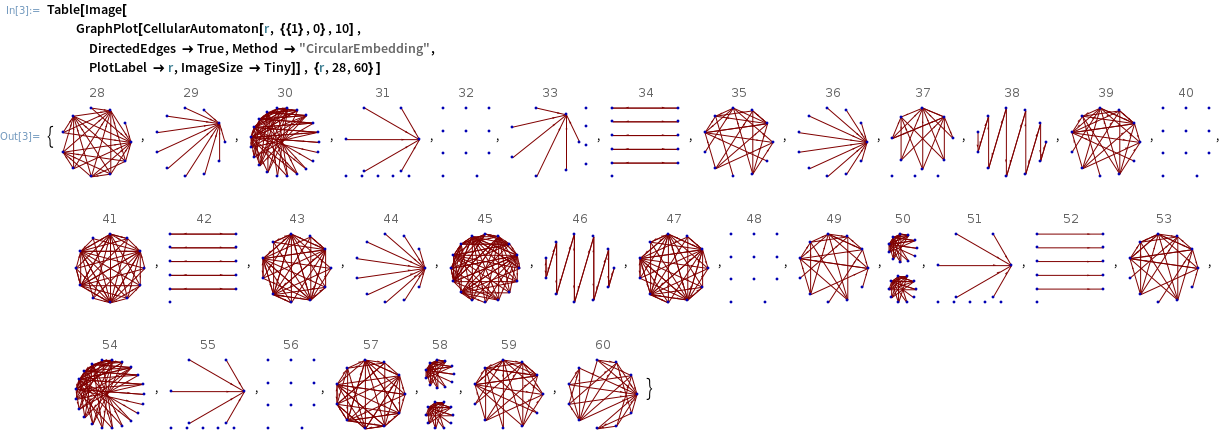
Table[Image[
   GraphPlot[CellularAutomaton[r, {{1}, 0}, NumberOfSteps],
    DirectedEdges -> True, Method -> "SomeGraphMethod",
    PlotLabel -> r, ImageSize -> Medium]], {r, 0, 255}];
Running this on 10 iterations in directed graphs utilizing "CircularEmbedding" yields a pretty interesting collection of graphs, a snapshot of which is seen below:
By combining several variations of the above code with the ImageCollage function, we can produce eight collections of all possible graph methods on all possible 1D elementary cellular automata:
CASteps = 10;

CE = Table[Image[GraphPlot[CellularAutomaton[r, {{1}, 0}, CASteps],
     DirectedEdges -> True, Method -> "CircularEmbedding",
     PlotLabel -> r, ImageSize -> Medium]], {r, 0, 255}];
SprEE = Table[Image[GraphPlot[CellularAutomaton[r, {{1}, 0}, CASteps],
     DirectedEdges -> True, Method -> "SpringElectricalEmbedding",
     PlotLabel -> r, ImageSize -> Medium]], {r, 0, 255}];
SprE = Table[Image[GraphPlot[CellularAutomaton[r, {{1}, 0}, CASteps],
     DirectedEdges -> True, Method -> "SpringEmbedding",
     PlotLabel -> r, ImageSize -> Medium]], {r, 0, 255}];
RD = Table[Image[GraphPlot[CellularAutomaton[r, {{1}, 0}, CASteps],
     DirectedEdges -> True, Method -> "RadialDrawing",
     PlotLabel -> r, ImageSize -> Medium]], {r, 0, 255}];
LD = Table[Image[GraphPlot[CellularAutomaton[r, {{1}, 0}, CASteps],
     DirectedEdges -> True, Method -> "LayeredDrawing",
     PlotLabel -> r, ImageSize -> Medium]], {r, 0, 255}];
LDD = Table[Image[GraphPlot[CellularAutomaton[r, {{1}, 0}, CASteps],
     DirectedEdges -> True, Method -> "LayeredDigraphDrawing",
     PlotLabel -> r, ImageSize -> Medium]], {r, 0, 255}];
HDE = Table[Image[GraphPlot[CellularAutomaton[r, {{1}, 0}, CASteps],
     DirectedEdges -> True, Method -> "HighDimensionalEmbedding",
     PlotLabel -> r, ImageSize -> Medium]], {r, 0, 255}];
SpiE = Table[Image[GraphPlot[CellularAutomaton[r, {{1}, 0}, CASteps],
     DirectedEdges -> True, Method -> "SpiralEmbedding",
     PlotLabel -> r, ImageSize -> Medium]], {r, 0, 255}];

ImageCollages = Table[Show[ImageCollage[g[[1]], Method -> "Rows"], PlotLabel -> g[[2]], LabelStyle -> Bold],
    {g, {{CE, "C I R C U L A R   E M B E D D I N G"}, {SprEE, "S P R I N G   E L E C T R I C A L   E M B E D D I N G"},
    {SprE, "S P R I N G   E M B E D D I N G"}, {RD, "R A D I A L   D R A W I N G"},
    {LD, "L A Y E R E D   D R A W I N G"}, {LDD, "L A Y E R E D   D I G R A P H   D R A W I N G"},
    {HDE, "H I G H   D I M E N S I O N A L   E M B E D D I N G"}, {SpiE, "S P I R A L   E M B E D D I N G"}}}];
The images produced were rather big so I decided to export and upload all of them into this Imgur album. I think it would be neat to see what kinds of neat things people are able to deduce from the images. I will continue to analyze the produced graphs and post any findings as a reply to this thread. This is my first post to the Wolfram Community, and hopefully the first of many more to come!


