Introduction
Here we wanted to measure properties such as volume and area of certain organs or unusual radiographic objects (e.g. tumors) in human CT scan using Wolfram Mathematica language. Properties measurement is important especially in tumors, as accurate estimation of tumor size is taken into consideration during treatment assignment, evaluation of treatment effectiveness and prediction of its outcomes. Several approaches have been used to determine the objects sizes in CT scan. Those are uni-dimensional and bi-dimensional measurements, identification of cross sectional area and volume. There is a large discussion in the literature on comparison of this measurement techniques as well beneficence of one from another. Some studies suggest that the use of the three-dimensional measurements are beneficial, other did not find significant additional benefit of volume calculation compared to uni-dimensional and bi-dimensional measurements. However, a study conducted by the Hopper et al. showed substantial interobserver variation in radiologists that perform CT linear object measurement, particularly for ill-defined and irregular lesions.
Our thought process towards the implementation started with the review of the literature on current practices in 3D recognition in CT scan images and reconstruction of the 3D images from existing CT scan data. Then we have started the process of recognition of objects first in 2D format and later in 3D format with measurement of the properties such as volume, shape parameters of the identified objects.
- Image Segmentation
- Image Reconstruction in 2D, 3D
First, we have imported and cropped human chest CT scan images and reconstructed them as 3D image.
listofImages =
Import["FilePath"];

listCroped = ImageCrop[#, {400, 400}] & /@ listofImages;

img3D = Image3D[listCroped]
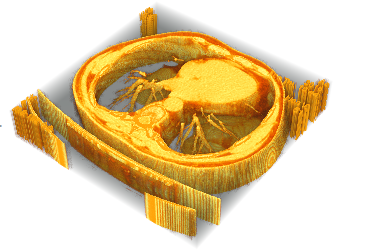
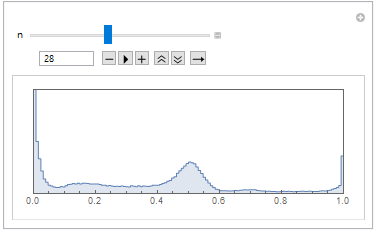
Then we have made the image histogram, where we can see that objects on the CT scan have different gray scale values, thus we will be able to distinguish different object by binarization operation.
Manipulate[
 listCroped[[n]] // ImageHistogram, {n, 1, Length[listCroped], 1}]
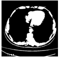
Here we perform the binarization using the MorphologicalBinarize function.
FillingTransform@
 DeleteSmallComponents[ImageSubtract[
   MorphologicalBinarize[listCroped[[17]], {.46, .55}],
   MorphologicalBinarize[listCroped[[17]], {.4, 1}]], 50]
2 D Components
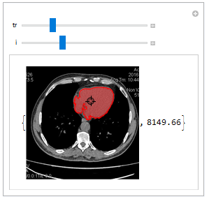
We have started with the delineation of objects in 2D images. For that purpose, we perform Morphological binarization.Then we extracted the morphological components of the preprocessed image. Applying the function MorphologicalComponents we have created a matrix that transformed every pixel of each component to an integer. Than we selected that component which has the same label for a certain position. This is implemented in selectCompOneSlice function .
selectCompOneSlice[pts_, img_, treshold_] := Module[
  {temp, mi, comp},
  temp = FillingTransform[MorphologicalBinarize[img, treshold], 2];
  mi = Image[MorphologicalComponents[temp]];
  comp = SelectComponents[mi, "Label",
    MemberQ[PixelValue[mi, #] & /@ Round@pts, 1. #] &]]
The function coputeComponetProp compuetes the area of the spectfied component and uses pixelToArea function to compute area in mm^2
pixelToArea[pxct_] := Module[
  {realsize = {428, 428},
   imgsize = {512, 512},
   pixelsize}, pixelsize = N[realsize/imgsize];
  (Times @@ pixelsize)*pxct]

coputeComponetProp[comp_] := Module[{area = 0},
  If[Length@ComponentMeasurements[comp, "Area"] != 0,
   area =
    pixelToArea[(1 /.
       First@ComponentMeasurements[comp, "Area"])];(*in mm^2*)];
  area]
Here you can see the demonstration of component selection and area measurement of every CT scan slice.
Manipulate[
 {HighlightImage[listCroped[[i]],
   selectCompOneSlice[{p}, listCroped[[i]], {tr, tr + 0.1}]],
  coputeComponetProp@
   selectCompOneSlice[{p}, listCroped[[i]], {tr, tr + 0.2}]},
 {{p, {1, 1}}, Locator}, {tr, 0.3, 0.8, 0.02}, {i, 1,
  Length[listCroped], 1}]
3D components
Than we proceeded to delinting objects on 3D. For that purpose, we have constructed interactive tool which could identify the desired object and manually marked it and then, extract properties for every slice.
slices = Length[listCroped];
pts = {}; tresholds = {};

DynamicModule[
 {points, i = 1, treshold, tresholdWidth},
 Table[points[j] = {}, {j, slices}];
 Table[treshold[j] = 0.4, {j, slices}];
 Column[{
   Slider[Dynamic[treshold[i]], {0.1, 0.8, 0.01},
    Appearance -> "Labeled"],
   Slider[Dynamic[tresholdWidth], {0.1, 0.2, 0.01},
    Appearance -> "Labeled"],
   Row[{Slider[Dynamic[i], {1, slices, 1}, Appearance -> "Labeled"],
     Button["+1", i = Min[i + 1, slices]],
     Button["-1", i = Max[i - 1, 1]],
     Button["+10", i = Min[i + 10, slices]],
     Button["-10", i = Max[i - 10, 1]],
     Button["Add point and threshold",
      (AppendTo[pts, First@points[i]];
       AppendTo[tresholds, treshold[i]])
      ]
     }],
   Dynamic[Row[{
      LocatorPane[
       Dynamic[points[i]],
       Image[MorphologicalBinarize[
         listCroped[[i]], {treshold[i], treshold[i] + tresholdWidth}],
         ImageSize -> 400],
       LocatorAutoCreate -> True
       ],
      Framed@
       Column[Flatten[
         Thread /@
          Select[{#, points[#]} & /@ Range[slices],
           Length[#[[2]]] > 0 &], 1], Alignment -> Top]
      }]]
   }]
 ]

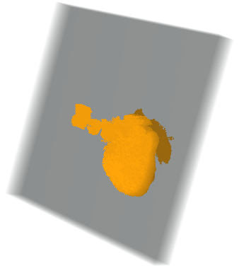
Here we constructed the 3D of the CT scan object under the interest, which in this case represents heart. Then, we computed the volume of the constructed object.
heart = Image3D@
  Table[selectCompOneSlice[{pts[[i]]},
    listCroped[[i]], {tresholds[[i]], tresholds[[i]] + 0.1}], {i, 1,
    Length[pts], 1}]
computeVolume[img3D_] :=
  Plus @@ (coputeComponetProp[#] & /@ Image3DSlices[img3D]);(*in mm^3*)

computeVolume[heart]

275395