Abstract
The aim of the project is to Analyze various differing musical(audio) waves and try to extract features and information, relevant for creating animations that conform to the tempo, genre, progression and other essential properties of music. To put it more simply the final goal is to create a visual representation of the musical file such that it transfers all the necessary information about that audio in an appealing and fun way. Various Machine learning and Audio processing algorithms are used in order to acquire the data from the audio.
Dataset generation
Not to overcomplicate things we simply use the example audios provided by Wolfram Alpha after putting some basic conditions of similarity and constraints for their acquisition.
data = Select[ExampleData["Audio"], 10 < ExampleData[#, "Duration"] < 15 &];
audioFiles = ConformAudio[AudioNormalize@AudioChannelMix[#, 1] & /@ ExampleData[#, "Audio"] & /@ data, SampleRate -> 11025];
Data and Feature extraction
For the initial steps of data acquisition we proceed with finding the elementary features such as the Mean, Standard Deviation, Skewness and Kurtosis
moments[mFile_] := Module[{file = mFile},
  mean = Mean[file];
  std = StandardDeviation[file];
  skewness = Mean[(file - mean)*3]/(std*3);
  kurtosis = Mean[(file - mean)*4]/(std*4);
  file = {mean, std, skewness, kurtosis};
  file
  ]
After looking at the initial features and getting some basic idea about what the waves look like we can proceed to finding some more detailed information. For this very purpose mathematica has a great function AudioMeasurments.
AudioFitList =
AudioMeasurements[#, {"ApproximateMedian", "Channels", "CrestFactor", "Duration", "Energy", "Length", "Loudness", "Max", "MaxAbs", "Mean",
"Median", "Min", "MinAbs", "MinMax",  "MinMaxAbs", "PeakToAveragePowerRatio", "Power", "RMSAmplitude", "SampleRate",
 "SpectralCentroid", "SpectralCrest",  "SpectralFlatness", "SpectralKurtosis", "SpectralRollOff", "SpectralSkewness",
 "SpectralSlope", "SpectralSpread",  "StandardDeviation", "TemporalCentroid", "Total",  "ZeroCrossingRate", "ZeroCrossings"}
, "List"] & /@ audioFiles;
We would also need to compute the properties locally for partitions of audio in order to get a Time Series about the corresponding properties
FullDatasetFeatures = AudioLocalMeasurements[#, { "Mean", "Median", "StandardDeviation", "SpectralCentroid",
      "SpectralSpread", "SpectralKurtosis", "Entropy", "RMSAmplitude",  "Power", "Loudness", "TemporalCentroid", "ZeroCrossingRate",
      "FundamentalFrequency", "HighFrequencyContent"
      }, "Dataset"] & /@ audioFiles;
Also for our further needs lets find the MFCC (Mel-frequency cepstral coefficients).
mfcc = AudioLocalMeasurements[#, "MFCC", PartitionGranularity -> {.05, .01}]["Values"] & /@ audioFiles
To Learn more about MFCC and other features look at the links provided in the References.
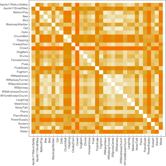
Defining a Metric Space For Computing Distance Between Audios
At the last point of the previous section we extracted the MFCC's of the whole dataset for the very purpose of defining the distance between 2 audio files.
ticks = Thread[{Range[Length@data], Text /@ data[[All, 2]]}];
MatrixPlot[DistanceMatrix[mfcc], ImageSize -> Large,  FrameTicks -> {ticks, Apply[Rotate[#, Pi/2] &, ticks, {2}]}]
Lets observe what the Heat Map looks like for our dataset.
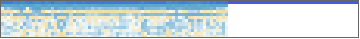
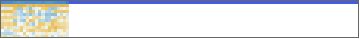
Other way of representation.
Column[MatrixPlot[#, PlotTheme -> "Minimal", ImageSize -> Medium] & /@Transpose /@ mfcc[[1 ;;2]]]
We take the first 2 audios as an example.
Clustering The Data
Now as we have nearly all features (some will be seen in further paragraphs) we can try to segment the dataset into different clusters. Lets call the classes that we acquire genres.
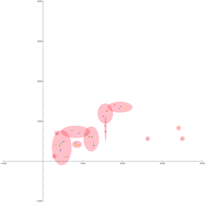
Initially I tried to use only 2 features( SpectralSpread, SpectralCentroid) in order to segment the data.
testFeatures = AudioMeasurements[#, {"SpectralCentroid", "SpectralSpread"}, "List"] & /@ audioFiles;
I anticipated the clustering to be quite troublesome using only these 2 features, however my concerns were unfounded as the clusters turned out to be quite well segmented.
Now as for clustering i used different algorithms e.g. DBSCAN, MeanShift etc etc. As the result were quite similar i decided to use the auto-selected method by Mathematica . To learn more about DBSCAN, MeanShift and others look up the links in the reference section.
clusters1 = FindClusters[props, Method -> "MeanShift"];
clusters2 = FindClusters[props, Method -> "DBSCAN"];
clusters = FindClusters[props];
We have to define an alternative standard deviation function, that can take one element or no elements, to use the three-sigma rule while plotting the found clusters.
stDev[x_List] := StandardDeviation[x]  /; Length[x] > 1
stDev[x_List] := 20 /; Length[x] == 1
stDev[x_List] := 0 /; Length[x] == 0


ListPlot[Partition[testFeatures, 1], PlotMarkers -> Automatic, ImageSize -> Full,
 Prolog -> ({Opacity[.3, RGBColor[1, 0.2, 0.3]], Disk[Mean@#, 3 stDev[#]] & /@ clusters}),
 PlotRange -> {{-1000, 4000}, {-1000, 4000}}, AspectRatio -> 1]
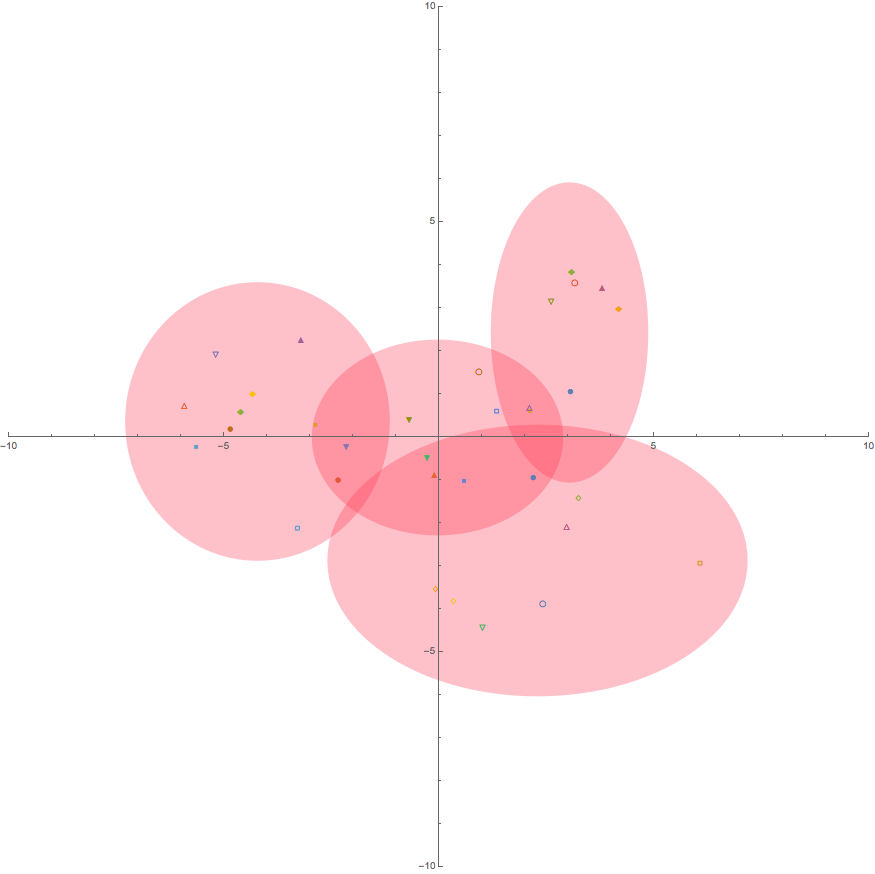
Now after testing it for only 2 features lets try using all the features and understanding which specific features are more important for clustering. For that very purpose we can use Dimensionality reduction algorithm such as PCA(Principal Components Analysis) and apply the clustering technique afterwards.
FullClusterd = FindClusters[DimensionReduce[(Flatten /@ AudioFitList), 2], 4];
As you can see i created 4 clusters and thats not a mere coincidence. I intend to have 4 varying animations conforming to each cluster of audios.
Now lets create a visualisation for the newly acquired clusters.
ListPlot[Partition[DimensionReduce[(Flatten /@ AudioFitList), 2], 1],
PlotMarkers -> Automatic, ImageSize -> Full,
 Prolog -> ({Opacity[.3, RGBColor[1, 0.2, 0.3]],
    Disk[Mean@#, 2.5 stDev[#]] & /@ FullClusterd}),
 PlotRange -> {{-10, 10}, {-10, 10}}, AspectRatio -> 1]
Now after the conventional way of visualization lets create some more fancy ways to portray the clusters.
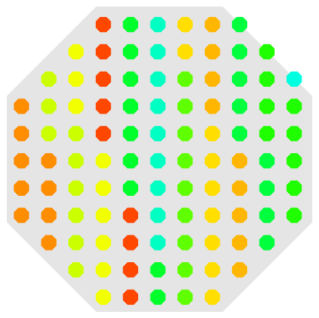
Method 1 and 2: Hexagonal Clustering
Method 1
1) Create a grid that we will use for populating with clusters.
grid = Table[{i, j}, {i, -10, 10, Length[audioFiles]/20}, {j, -10, 10, Length[audioFiles]/20}]
2) Create a base Polygon and a rule for finding elements inside that Octagon.
ocatag = RegularPolygon[{0, 0}, 10, 8]
requiredPart = RegionMember[RegularPolygon[{0, 0}, 10, 8]]
3) Populate the clusters inside the base Octagon with octagons of differing colours.
k = Length[Normalize@(Mean /@ Flatten /@ clusters)];
gridClust[k_] := Module[{part, hues, polyg, polygLen, repetedHues},
  part = Range[1, k];
  hues = Hue /@ (Normalize[Mean /@ Flatten /@ clusters][[part]]);
  polyg =  RegularPolygon[#, 0.5, 8] & /@ Select[(# & /@ Flatten[grid, 1]), requiredPart];
  polygLen = Length@polyg;
  repetedHues = Flatten[ Transpose@Table[hues, {i, polygLen/(Length@hues) + 1}]][[;;polygLen]];
  Graphics[{{Opacity[0.1], RegularPolygon[{0, 0}, 10, 8]},
    Transpose@{repetedHues, polyg}
    }]
  ]
gridClust[k]
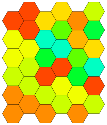
Method 2
1) Create a hexagonal connected mosaic and Colour them proportionally with respect to elements of the cluster.
part = Range[1, k];
hues = Hue /@ (Normalize[Mean /@ Flatten /@ clusters][[part]]);
h[x_, y_] :=  Polygon[Table[{Cos[2 Pi k/6] + x, Sin[2 Pi k/6] + y}, {k, 6}]]
repetedHues = Flatten[ Transpose@Table[hues, {i, 32/(Length@hues) + 1}]][[;; 32]];
hex = Graphics[
  {EdgeForm[Opacity[.7]],
   Table[
    {repetedHues[[Mod[i*j, Length[repetedHues]]]],
     h[3 i + 3 ((-1)^j + 1)/4, Sqrt[3]/2 j]},
    {i, 3}, {j, k}
    ]
   }
  ]
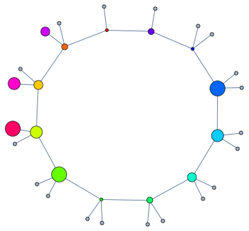
Method 3 Cluster Visualisation with Graph
Graph[Table[Property[v, {VertexSize -> 0.2 + 0.2 Mod[v, 5], VertexStyle -> Hue[v/15, 1, 1]}], {v, 0, 14}],
Table[v <-> Mod[v + 1, k],{v,0,Length[audioFiles]}]]
At Last!!!! Lets start to make an animation
Firstly as mentioned above lets extract the last set of features from the music file using the Fourier Transform. We can acquire the frequency/power spectrums using a custom function.
fftGeneralFeatures[wavData_] := Module[ {data = wavData},
  furierTrans = Fourier[data];
  data = furierTrans;
  amount = ((Length[data]/2) + 1);
  data = data[[2 ;; amount]];
  data = Abs[data];
  totalPower = Total[data];
  data = Partition[data, 10];

   For[i = 1, i <= Length[data], i++,
   feature = Total[data[[i ;; i]]/totalPower];

   ] ;
  feature
  ]
After we have a function to calculate the Fourier generated features of and audio file, we must proceed to preprocessing that audio file in order to create an animation dependent on its features.
Preprocessing
(We are going to write functions and modules for everything)
1) Firstly we want to get the duration of the whole audio file.
roundedLengthOfAudio[audio_] := Ceiling[AudioMeasurements[audio, "Duration"]];
2) After that we retrieve the samples from the whole audio and further divide them into chunks.
preprocess[audioWave_] :=
  Module[{audio = audioWave, audioData, audioChunks, length},
   length = roundedLengthOfAudio[audio];
   audioData = Flatten[AudioData[audio]];
   audioChunks = Partition[audioData, Ceiling[AudioMeasurements[exampleAudio, "SampleRate"] / length]]; (*every second*)
   audioChunks
   ];
3) After preprocessing we write functions to derive the features with Fourier.
fourierSpectrumFrequency [audioData_] := Abs[Fourier[audioData]];
chunkPart[audioWaveData_, part_] :=  fourierSpectrumFrequency[preprocess[audioWaveData][[part]]];
4) When feature extraction is complete we have to interpolate the Fourier data for each of the chunks to create functions that we will use for the animation.
int[audioWaveData_, part_] :=  Interpolation[chunkPart[audioWaveData, part], x];
squeesedInt[audioWaveData_, part_] :=  Rescale[Interpolation[chunkPart[audioWaveData, part]][x + Pi], {0, 10}, {0, Pi}];
 (*squeesing for spherical 3D plot*)
5) Store the core info about the wave into variables.
chunkAmount = Dimensions[preprocess[exampleAudio]][[1]];
chunkLength = Dimensions[preprocess[exampleAudio]][[2]];
sampleRate = Ceiling[AudioMeasurements[exampleAudio, "SampleRate"]];
6) Assemble all of the interpolating functions in 1 variable. (Good for optimising the speed of 3d Plot creation)
evaluator = Table[int[exampleAudio, part], {part, 1, chunkAmount}];
7) Create the 1'st type of animation. (The parameters are set to create the 3D plots fast, However for smoother and higher quality resulting animation they should be changed)
list = Table[
   RevolutionPlot3D[evaluator[[part]], {x, 2, 8},
    ColorFunction -> (ColorData["Rainbow"][#6] &),
    PlotStyle -> Directive[Opacity[0.7], Specularity[White, 10]],
    Mesh -> None, PlotPoints -> 20, PerformanceGoal -> "Speed",
    Boxed -> False, Axes -> False, SphericalRegion -> True,
    Lighting -> "Neutral"],
   {part, 1, chunkAmount, 1}
   ];
8) Export is as a gif. (Or a vide format such as avi/mov)
Export["example.gif", list, "DisplayDurations" -> {0.225}]; (*0.225 is chose as an example*)
9) Assemble all of the interpolating functions in 1 variable. (Now we use the squeesedInt for the 2'nd animation)
evaluator2 = Table[squeesedInt[exampleAudio, part], {part, 1, chunkAmount}];
10) Create the 2'nd type of animation. (The parameters are set to create the 3D plots fast, However for smoother and higher quality resulting animation they should be changed)
secondList = Table[
   SphericalPlot3D[evaluator2[[part]], {x, 0, Pi}, {\[Phi], 0, 2 Pi},
    ColorFunction -> (ColorData["Rainbow"][#6] &),
    PlotStyle -> Directive[Opacity[0.7], Specularity[White, 10]],
    Mesh -> None, PlotPoints -> 15, PerformanceGoal -> "Speed" ,
    Boxed -> False, Axes -> False, SphericalRegion -> True],
   {part, 1, 100}
   ];
11) TADAAAAA Done
PS: Observe some results

PSS: The Animations can be drastically improved if more frame are taken on smaller audioChunks.(They just take a lot of time to create)
References
Audio Signal Processing
MFCC Info
DBSCAN
DBSCAN_Wiki
Mean Shift technique
Fourier Transform
Principal Component Analysis


