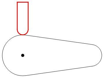
I helped to answer a camshaft question and thought I'd share the code here too. A camshaft is a shaft to which a cam is fastened or of which a cam forms an integral part. The goal is to make the valve tap the cam throughout the course and produce an image similar to the one below.

Here is the cam provided by the OP.

r1 = 15; r2 = 8; c = 50; ? = ArcSin[(r1 - r2)/c] // N;

l1 = (2 ? + ?) r1;
l2 = (? - 2 ?) r2;
l3 = 2 c Cos[?];
L = 2 c Cos[?] + (2 ? + ?) r1 + (? - 
      2 ?) r2;

cam = {Circle[{0, 0}, r1, {Pi/2 - ?, ((3*Pi))/2 + ?}], 
   Circle[{c, 0}, r2, {Pi/2 - ?, -(Pi/2) + ?}], 
   Line[{{Cos[Pi/2 - ?]*r1, 
      Sin[Pi/2 - ?]*r1}, {Cos[Pi/2 - ?]*r2 + c, 
      Sin[Pi/2 - ?]*r2}}], 
   Line[{{Cos[((3*Pi))/2 + ?]*r1, 
      Sin[((3*Pi))/2 + ?]*r1}, {Cos[-(Pi/2) + ?]*r2 + c,
       Sin[-(Pi/2) + ?]*r2}}], PointSize[0.03], Point[{0, 0}]};

g = Graphics[cam];

rValve = 4;
posição = 15 + rValve;
valve = Graphics[
   {
    Red,
    Thickness[0.008],
    Circle[{0, posição}, rValve, {0, -Pi}],
    Line[{{-rValve, posição}, {-rValve, posição + 20}}],
    Line[{{rValve, posição}, {rValve, posição + 20}}],
    Line[{{-rValve, posição + 20}, {rValve, posição + 20}}]
    }
   ];

Show[g, valve]

To solve this, RegionDistance can be useful here.

cambd = RegionUnion[
  Circle[{0, 0}, r1, {Pi/2 - ?, ((3*Pi))/2 + ?}], 
  Circle[{c, 0}, r2, {-(Pi/2) + ?, Pi/2 - ?}], 
  Line[{{Cos[Pi/2 - ?]*r1, Sin[Pi/2 - ?]*r1}, {Cos[Pi/2 - ?]*r2 + c, Sin[Pi/2 - ?]*r2}}], 
  Line[{{Cos[((3*Pi))/2 + ?]*r1, Sin[((3*Pi))/2 + ?]*r1}, {Cos[-(Pi/2) + ?]*r2 + c, Sin[-(Pi/2) + ?]*r2}}]
];

posiçãoVal[?_?NumericQ] :=
  With[{cambd? = TransformedRegion[cambd, RotationTransform[?]]},
     y /. Quiet[FindRoot[RegionDistance[cambd?, {0, y}] == rValve, {y, 60}]]
  ]

Table[posiçãoVal[?], {?, 0, 2? - ?/6, ?/6}]

{19., 20.4853, 30.8282, 62., 30.8282, 20.4853, 19., 19., 19., 19., 19., 19.}

frames = Table[
  Graphics[{
    GeometricTransformation[cam, RotationMatrix[?]],
    posição = posiçãoVal[?];
    {Red, Thickness[0.008], 
     Circle[{0, posição}, rValve = 4, {-Pi, 0}], 
     Line[{{-rValve, posição}, {-rValve, posição + 20}}], 
     Line[{{rValve, posição}, {rValve, posição + 20}}], 
     Line[{{-rValve, posição + 20}, {rValve, posição + 20}}]}
   },
   PlotRange -> {{-59, 59}, {-59, 83}}
  ],
  {?, 0, 2? - ?/12, ?/12}
];

Export["Desktop/cam.gif", frames];

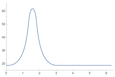
Here's a plot of the valve height relative to the cam center point:

Plot[posiçãoVal[?], {?, 0, 2?}, PlotRange -> {15, 66}, PerformanceGoal -> "Speed"]

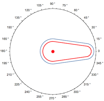
In polar coordinates, we can see we're indeed tracing the isocurve of distance 4 from the cam:

Show[
  PolarPlot[posiçãoVal[?+?/2], {?, 0, 2?}, PolarAxes -> {True, False}, PolarTicks -> {"Degrees", Automatic}, PerformanceGoal -> "Speed"],
  Graphics[{Red, Thick, cam}]
]