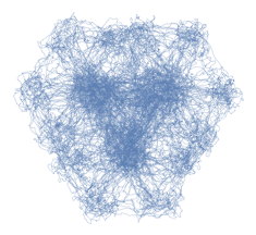
I am attempting to extrapolate this 2d plot to a 3d plot, since it seems to hint at an interesting 3d structure.

ParametricPlot[
 Sum[{1/2^(k/3) Sin[2^(k/3) t], (-1)^k/2^(k/3) Cos[2^(k/3) t]}, {k, 0, 30}]
 , {t, 0, 500}, Axes -> False, PlotPoints -> 2000, MaxRecursion -> 5,  PlotStyle -> Thickness[0.001]]

Note: Taking t higher gives a more detailed plot: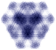

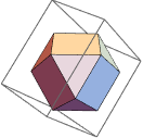
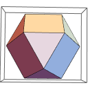
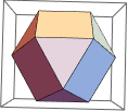
I imagine the result would look similar to one of the following, with the curve filling out the interior of the shape in some interesting way.

PolyhedronData["Cuboctahedron"]
PolyhedronData["TriangularCupola"]
PolyhedronData["TriangularOrthobicupola"]

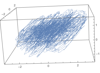
So far I've tried many candidates for the z coordinate, but all of them yield a messy result. For instance:

xx[kay_] := Sum[1/2^(k/3) Sin[2^(k/3) t], {k, 0, kay}];
yy[kay_] := Sum[(-1)^k/2^(k/3) Cos[2^(k/3) t], {k, 0, kay}];
zz[kay_] :=   Sum[ 1/2^(k/3) Sin[2^(k/3) t] Cos[2^(k/3) t], {k, 0, kay}];

hyperlattice3D[a_, tee_, plotpts_] := ParametricPlot3D[
  {xx[a], yy[a], zz[a]}
  , {t, 0, tee 2 Pi}, AspectRatio -> Automatic, PlotRange -> All, 
  PlotPoints -> plotpts, MaxRecursion -> 5,  PlotStyle -> Thickness[0.001]]

hyperlattice3D[30, 50, 300]

Any ideas for a natural choice of the z-coordinate which yields a cool-looking plot?