Center of Mass

This is another one with some interesting math hiding behind it. The starting point is very simple: 24 equally-spaced points on the unit circle.

Now, think of the circle as the extended real numbers (i.e., the reals plus a point at infinity). Concretely, we can think of mapping the real line to the circle by inverse stereographic projection. Under this correspondence, the scaling transform $x \mapsto a x$ pushes points on the circle up towards the north pole or down towards the south pole depending on whether $a>1$ or $a<1$.

As $a \to \infty$, all of the 24 points except the one at the south pole limit to the north pole, which is the starting point of the animation. The animation then shows what happens as $a$ gets smaller and eventually limits to 0. All the points except the one trapped at the north pole now limit to the south pole.

The point in the middle of the circle is the center of mass of the 24 points. Each of the 24 points is connected to the center of mass by an arc of a circle which is perpendicular to the unit circle at the points where they intersect. In other words, thinking of the unit disk as the Poincaré disk model of the hyperbolic plane, the circle arcs are the geodesic rays from the center of mass out to each of the 24 points on the circle at infinity.

In this hyperbolic interpretation, the scaling transform $x \mapsto a x$ corresponds to a hyperbolic isometry. The isometry group of the hyperbolic plane is $PSL(2,\mathbb{R})$, the projective special linear group (i.e., the group of $2 \times 2$ real matrices with determinant 1 modulo the equivalence relation $A \sim -A$). Thinking of points in the unit disk as complex numbers $z$ of modulus less than 1, the action of $PSL(2,\mathbb{R})$ is by fractional linear transformations of the special form $z \mapsto \frac{\alpha z + \beta}{\bar{\beta}z + \alpha}$.

So here's the code. First of all, a function which inputs a point in the disk, a complex number $z$, and a parameter $t$ between 0 and 1, and outputs $\frac{\alpha z + \beta}{\bar{\beta}z + \alpha}$, where $\alpha$ and $\beta$ are chosen so as to send the point a fraction $t$ of the way to the origin. In other words, this gives the hyperbolic isometry corresponding to translation along the geodesic containing the origin and the given point. When the point is on the $y$-axis, this just corresponds (via stereographic projection) to scalings of the form $x \mapsto a x$.

ScaleCenter[point_, z_, t_] := Module[{?, ?},
   ? = Sqrt[1/(1 - t^2*Norm[point]^2)];
   ? = -t*(Complex @@ point)*?;
   (?*z + ?)/(Conjugate[?]*z + ?)
   ];

Next is code for hyperbolic geodesics between two arbitrary points in the Poincaré disk (or on its boundary). The idea is to use the relationship between the various models of the hyperbolic plane summarized in this Wikipedia image:

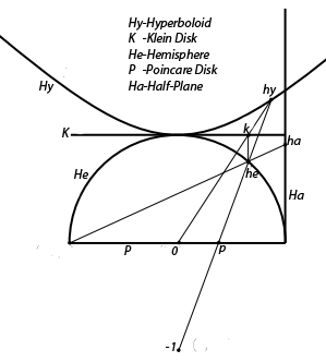
Essentially, I want to use the connection between the Poincaré model and the Klein model, since geodesics are easy in the Klein model: they're just straight lines. So what I want to do is map my points in the disk model to the Klein model, take the obvious parametrization of the line connecting them, then map back to the disk model.

Now, the mapping between the two models is conceptually straightforward: given a point in the Poincaré disk, inverse stereographically project to the sphere, then orthogonally project to the Klein disk. So here are the necessary functions:

Stereo[{x_, y_, z_}] := {x/(1 + z), y/(1 + z)};
InverseStereo[{x_, y_}] := {2 x/(1 + x^2 + y^2), 2 y/(1 + x^2 + y^2), (1 - x^2 - y^2)/(1 + x^2 + y^2)};
hypgeo[p1_, p2_, t_] := 
  Stereo[Append[#, Sqrt[1 - Norm[#]^2]]] &[(1 - t) InverseStereo[p1][[;; 2]] + t InverseStereo[p2][[;; 2]]];

And now, here's the Manipulate that puts it all together (I only let the parameter go from 0.001 to 0.999 because things blow up at 0 and 1):

DynamicModule[
 {cloud = Table[{Cos[a], Sin[a]}, {a, 0., 2 ? - 2 ?/24, 2 ?/24}],
  lim = 0.5,
  cols = RGBColor /@ {"#2E6E65", "#F4F7ED", "#86EE60", "#2B3752"},
  t, tcloud, c},
 Manipulate[
  t = -lim Cos[? u];
  tcloud = ReIm[ScaleCenter[{0, 1/lim}, Complex @@ #, t]] & /@ cloud;
  c = Mean[tcloud];
  Show[
   ParametricPlot[Evaluate[hypgeo[#, c, r] & /@ tcloud], {r, 0, 1}, 
    PlotStyle -> Directive[cols[[3]], Thickness[.00275]], Axes -> False],
   Graphics[{Thickness[.004], cols[[1]], Circle[], cols[[2]], 
       JoinForm["Round"], PointSize[.0125], Point /@ #} &[tcloud]],
   ImageSize -> {540, 540}, PlotRange -> 1.3, Background -> cols[[-1]]],
  {u, .001, .999}]
 ]