In other threads, we've seen some nice GIFs showing large amplitude motion of vibrating membranes. This author raised one objection, and here we present more details regarding possibilites in physical oscillators. For the sake of simplicity, we restrain ourselves to a one dimensional string, fixed at both ends. To apply numerical methods, the string is taken to be unit length $L=1$, unit stiffness $k_1=1$, and divided into 900 equal intervals of mass $m=1$. The applied tension at each interval is $ T = k_1|\partial{ \bf{x}} / \partial{s} | + k_3|\partial{ \bf{x}} / \partial{s} |^3$, in the same conventions as Large Amplitude Motion of a String. Time evolution is calculated by a sequence of iterated, symplectic maps using a second order integrator, as in Fourth Order Symplectic Integration . We could change parameters of the evolution algorithm--specifically: the number of divisions or the order of the integrator--to obtain better results, but these choices satisfy our convergence criteria. Now the code.

• One partial step along the Hamiltonian manifold

  SymplecticMap[qp_, cd_, ForceF_, dt_] := With[
  {p1 = qp[[2]] + cd[[1]]*ForceF[qp[[1]]]*dt},
  {qp[[1]] + cd[[2]]*p1*dt, p1}]
  

• Discrete Wave Time Evolver ( not used here )

  EvolveWave[Amp_, k1_, k3_, cdList_, NGrid_, dt_, time_] := NestList[
  Fold[SymplecticMap[#1, #2, Function[{a}, Forces[a, k1, k3, NGrid]],
  dt] &, #, cdList  ] &,
  IC[NGrid, Amp], time];
  

• Autocorrelation function

  AutoCorrelation[Amp_, k1_, k3_, cdList_, NGrid_, dt_, time_] := 
  With[{ic = IC[NGrid, Amp][[1, All, 2]]},
  Reap[Nest[(Sow[ #[[1, All, 2]].ic];
  Fold[ SymplecticMap[#1, #2, Function[{a}, Forces[a, k1, k3, NGrid]], dt] &, #, cdList  ]) &,
  IC[NGrid, Amp], time]][[2, 1]]/ic.ic ];
  

• String force function

  Forces[qs_, k1_, k3_, NGrid_] := Prepend[Append[
  Partition[qs, 3, 1] /. {x_, y_, z_} :> Plus[
  NGrid*Subtract[x, y]*(k1   + k3 #^2) &@(Norm[x - y]*NGrid),
  NGrid*Subtract[z, y]*(k1  + k3 #^2) &@(Norm[z - y]*NGrid)
  ], {0, 0}], {0, 0}]
  

• Initial Condition

  IC[NGrid_, Amp_] := {
  {#/(NGrid - 1), Amp Sin[2 Pi #/(NGrid - 1)]} & /@ 
  Range[0, (NGrid - 1)], Table[{0, 0}, {NGrid}]}
  

• Integrator Parameters

  CD2 = {{0, 1/2}, {1, 1/2}};
  CD3 = {{7/24, 2/3}, {3/4, -2/3}, {-1/24, 1}};
  CD4 = {{x + 1/2, 2 x + 1}, {-x, -4 x - 1}, {-x, 2 x + 1}, {x + 1/2, 
  0}} /. FindRoot[48 x^3 + 24 x^2 - 1, {x, 0.1756}];
  

Combining all of these functions and variables, we will determine the affect of anharmonicty $(k_3 \neq 0)$ in the small $ k\_{3} $, small amplitude limit. Throughout the computer experiment, $ k_3 $ takes values $( 0.000, 0.0025, 0.005, 0.0075, 0.01 )$, while amplitude goes in steps between $0$ and $L/2$.

First we check if our parameters are reasonable by plotting a makeshift stress strain graph

bound = NIntegrate[Sqrt[1 + (A 2 Pi Cos[2 Pi x])^2 ] /. A -> .5, {x, 0, 1}]
Show[
Plot[1 L - # L^3, {L, 0, 5}] & /@ {0.0 , 0.01, 0.0075, 0.005, 0.0025},
Graphics[{Dashed, Line[{{1, 0}, {1, 6}}], 
Line[{{bound, 0}, {bound, 6}}]}],
ImageSize -> 700]

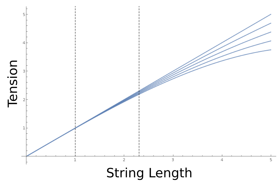
Where minimum and maximum excursions are marked by dashed lines. Next we plot the theoretical autocorrelation function, along with numeric estimates for maximum and minimum excursion with the largest $k_3=0.01$ .

AbsoluteTiming[ ACMinTest = AutoCorrelation[.001, 1, -0.01, CD2, 900, .01, 3300];]
Out[]= {114.863, Null}
AbsoluteTiming[ ACMaxTest = AutoCorrelation[.5, 1, -0.01, CD2, 900, .01, 3300];]
Out[]= {111.181, Null}

Show[
 Plot[Cos[2 Pi x], {x, 0, 1.1}, PlotStyle -> Directive[Thick, Red]],
 ListPlot[{100 #/3000, ACMaxTest[[100 #]]} & /@ Range[33], PlotStyle -> Directive[Thick, Blue]],
 ListPlot[{100 #/3000, ACMinTest[[100 #]]} & /@ Range[33],   PlotStyle -> Directive[Thick, Green]],
 ImageSize -> 500]

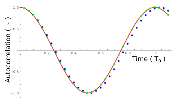
In this image, the horizontal units are in multiples of $T_0$, the harmonic period. Low energy solutions closely follow the harmonic prediction, but already at amplitude $L/2$ the affect of $k_3 \neq 0 $ is apparent as an increase in period of oscillation.

Finally, we map across amplitude values and $k_3$ values ( for about 1.5 hrs of personal computer time ), to obtain the following plot: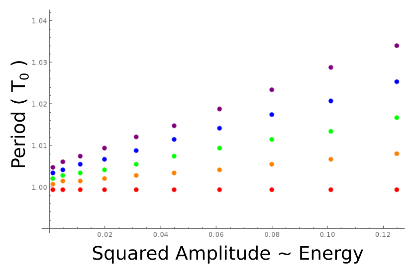

From this plot and a few quick linear fits, it becomes immediately apparent that $$ T = T_1(1+c_1 k_3 E+ . . .) ,$$ with $T_1$ a frequency near the harmonic.

• Remarkably, this is what we hoped to find!

The same low energy form as seen in a wide variety of one-dimensional oscillations, as per the derivation of Plane Pendulum and Beyond... (rejected by AJP only for being "Not of Interest"). We might as well throw out a wild conjecture to hunt down in 2017: could the form of the period expansion match at all orders of magnitude in energy? If the answer is provable yes, this is yet another nice result for building analogies between physical systems.

Now a three percent change in period may not seem like much, but consider that our experiment's maximum $k_3$ is only one percent of $k_1$. We can reasonably expect with $k_3$ ten percent of $k_1$ to see change of period above ten percent. Alternatively if we choose a large amplitude of something wild like $5L$ ( as far as I could tell from the code, this is around the value in one of the other posts), we should expect to see a huge jump in the period, possibly with quadratic, cubic, or higher energy dependence.

And watch out! If we're talking about a real drum, and you hit it that hard... It could break!

1. Before the sign out, radio check.
2. What's the frequency selector say?
3. It's Neu! German drums, Hallogallo!
4. Watch out, Listen up! German Strings!
5. If just one adventurer, [censored], lost
6. could find mistaken, lunatic Goethe
7. crowing his multicolored megabytes
8. in a revolutionary theory of sound.