Introduction

The summer just passed, I had the honor of attending the Wolfram High School Summer Camp at Bentley University. After returning, I needed to get my fix of the Wolfram language, so I applied for the Wolfram Mentorship Program. Dr. Rowland helped me work on creating new ways to visualize the patterns of the binaries of files, a sidetrack to Angela Chen's Summer School project.

File encodings are a wild breed of different patterns, headers, and footers. While hex editors are a mainstream way to analyze file structures, colorful visualizations can offer the same analysis in a more succinct and time-efficient way.

Basic ArrayPlot

A starting point was a standard array where every byte was represented by a square color-coded with a byte value of 0 corresponding with purple and a 255 byte as red. Below is an example of a simple 84,000 byte .stl file partitioned into rows of 800 file plot: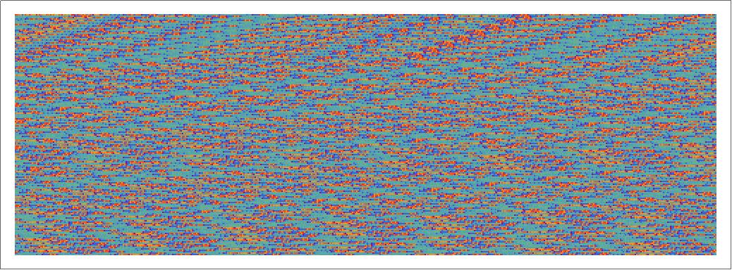
The ArrayPlot function with Partition constructs a matrix. The user is given the option of how many bytes (represented by squares) wide the visualization becomes as well as which color scheme to use and the size of the image produces. The Wolfram language has 51 built-in color schemes, but Rainbow was selected for the purposes of this demonstration because its wide variety of colors allows for a more detailed view of byte constructions. The issue with basic ArrayPlots is that the visualization changes based on the width selected and the size of the file. There is little consistency. A solution to this is arranging the bytes along a path defined by a FASS curve. Not only does this keep the representation stable across various file lengths, but it may also introduce new ways of thinking about the patters by offering a new way of looking at them. The two FASS curves chosen for this survey are the triangle and dragon curves.
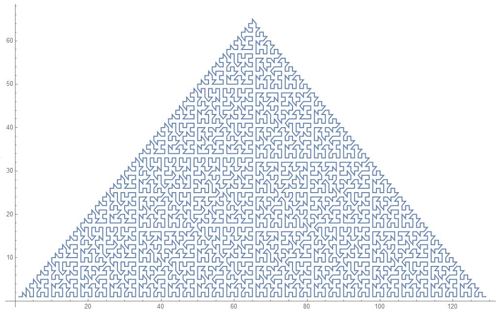
Triangle Curve
An L-system was used in order to produce the coordinates for both fractals. The rule used was X-> XF-F+F-XF+F+XF-F+F-X with X as the axiom. A “+” tells the program to rotate ?/2 radians counterclockwise while a “-“ makes a clockwise rotation of the same amount. “X” represents moving forward for one unit. “F” is essentially a placeholder. A function was written, which when given the amount of iterations, produced a list of coordinates for the triangle curve. The final line moves the graph above the x axis so that no coordinate contains 0 since matrices start from 1. A graph of the coordinates of seven iterations is shown here:

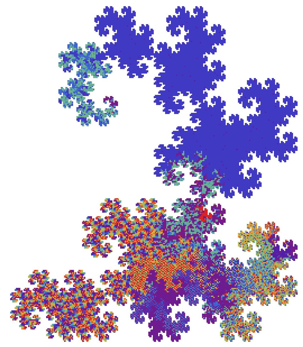
Dragon Curve
This was constructed using the same base code as the triangle curve, except with the L-system rules: X -> X+YF+ and Y -> -FX-Y.
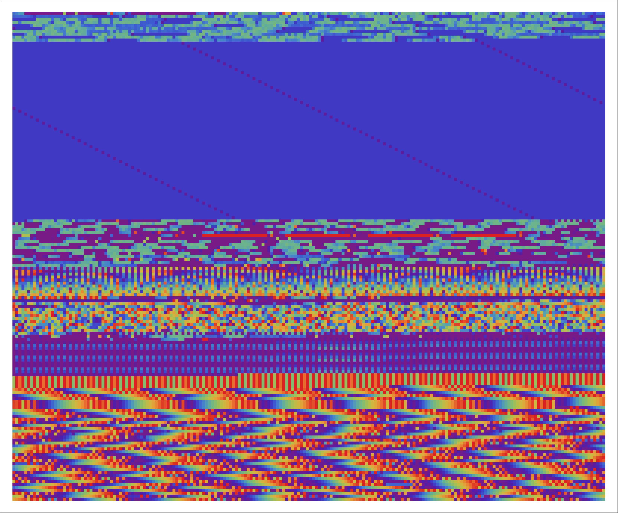
Comparison Between the Three Visualizations
Byte Array

Triangle

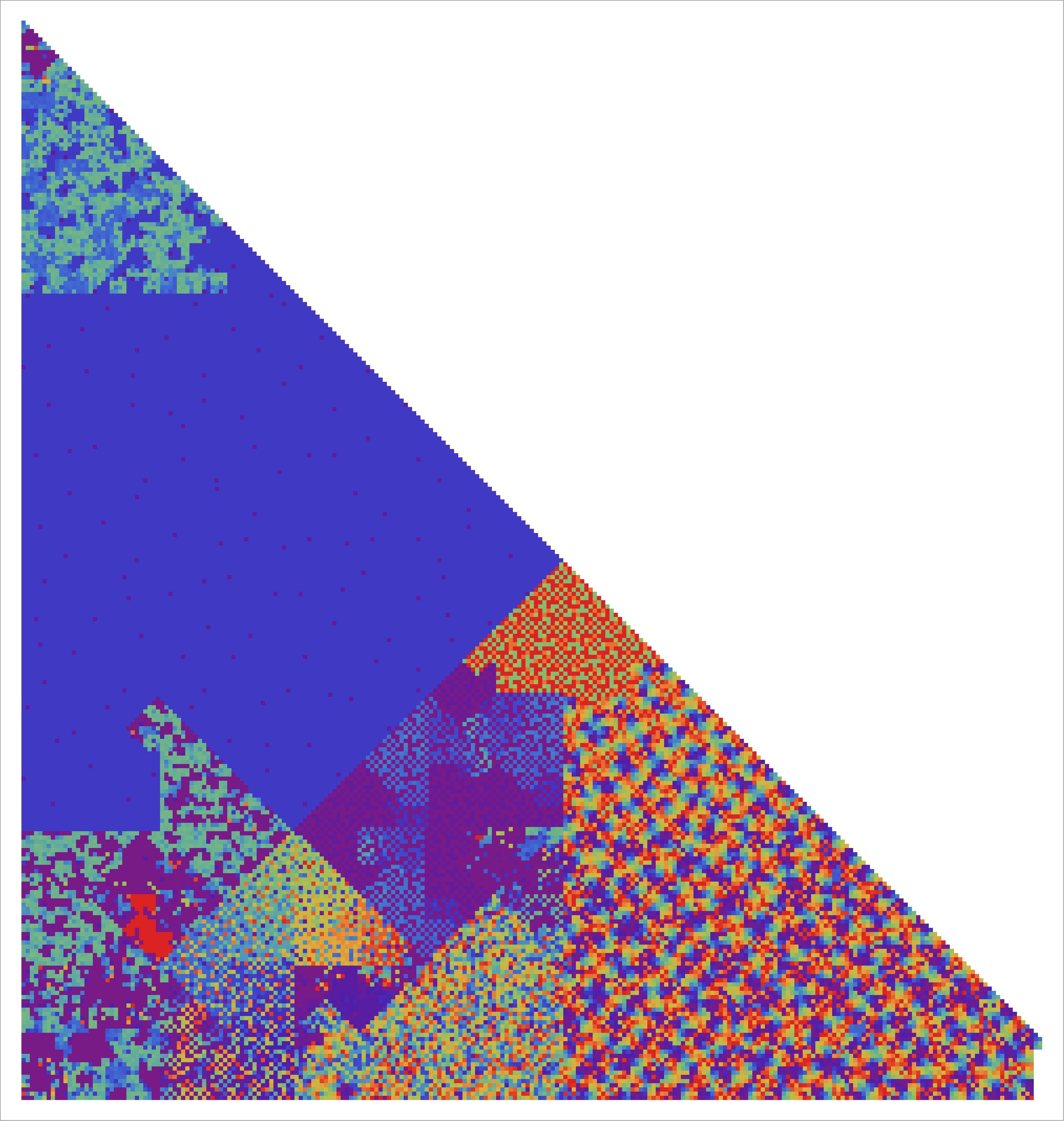
Dragon

These visualizations are amazing for comparing different file type structures. The full function is is the attached notebook, give it a try!

Options[ByteVisualization] = {FractalType -> "None", 
   GrayCode -> "False", Width -> 640, Max -> 33024, 
   ImageSize -> Medium, Background -> White, 
   ColorFunction -> "Rainbow"};

triangleCurve[size_Integer?Positive] :=
  triangleCurve[size] =With[{pos = DeleteDuplicates[
       Map[AnglePath,ReplaceAll[Characters[StringReplace[

            SubstitutionSystem[{"X" -> "XF-F+F-XF+F+XF-F+F-X"}, "X", 
             size], {"F" -> ""}]], {"+" -> {0, -Pi/2}, "-" -> {0, Pi/2}, "X" -> {1, 0}}]][[-1]]]}, 
    Transpose[Transpose[pos] - Min /@ Transpose[pos] + 1]];

dragonCurve[size_Integer?Positive] :=
  dragonCurve[size] =With[
    {pos = DeleteDuplicates[
       Map[AnglePath,ReplaceAll[Characters[StringReplace[

            SubstitutionSystem[{"X" -> "X+YF+", "Y" -> "-FX-Y"}, "FX",
              size], {"F" -> ""}]], {"+" -> {0, -Pi/2}, 
           "-" -> {0, Pi/2}, "Y" -> {1, 0}, 
           "X" -> {1, 0}}]][[-1]]]}, (*N for faster*) 
    Transpose[Transpose[pos] - Min /@ Transpose[pos] + 1]];

positionsdra = Round[dragonCurve[17]]; (*may adjust this value for larger files*)

positionstri = Round[triangleCurve[9]]; (*same here*)

ByteVisualization[data_, OptionsPattern[ByteVisualization]] :=

 Module[{positionsmore, triangleCurve, triview, 
   convertToPostGreyCodeDecimal, x, dragonCurve, n, data2 = data},
  convertToPostGreyCodeDecimal[x_] := 
   Replace[x, Thread[Range[0, 255] -> Experimental`GrayCode[8]]];
  If[OptionValue[GrayCode] == "True", 
   data2 = convertToPostGreyCodeDecimal /@ data];

  view2[l_List, n_List] := 
   ArrayPlot[
    SparseArray[{n[[;; Length[l]]] -> l + 1}, Automatic, 257], 
    ImageSize -> OptionValue[ImageSize], 
    ColorFunction -> OptionValue[ColorFunction], 
    ColorRules -> {257 -> OptionValue[Background]}];

  Which[
   OptionValue[FractalType] == "None", 
   ArrayPlot[
    Partition[data2[[;; OptionValue[Max]]], OptionValue[Width]], 
    ImageSize -> OptionValue[ImageSize], 
    ColorFunction -> OptionValue[ColorFunction]],

   OptionValue[FractalType] == "Triangle", 
   view2[data2[[;; OptionValue[Max]]], positionstri], 
   OptionValue[FractalType] == "Dragon", 
   view2[data2[[;; OptionValue[Max]]], positionsdra]
   ]]

Attachments: