Hi Gary,
I see two approaches you could take when adding the milk to the coffee. Either you could have everything collected into a single component that has a event in it corresponding to the addition of the milk, or you could have a separate component that specifies the addition of milk as a flow over time. I explored both those scenarios in the attached model. Would be very interesting to hear your input which one would be better from a teaching perspective.
Approach 1, with a discrete event in the coffee involves creating a copy of the HeatCapacitor component and adding some parameters that separates the heat capacity of the milk, the amount of milk added, when it is added, etc. As you say, the mixed Cp is unknown. A naïve initial approach could be to just add the two heat capacities together. If C is the total heat capacity of the coffee, with or without milk, you could add an equation that says:
C = if time > AddTime then Ccoffee * Vcoffee * 1000 + Cmilk * Vmilk * 1000 else Ccoffee * Vcoffee * 1000;
The coefficients are just there to convert the different units.
The temperature is a bit more difficult, since it varies continuously over time it is state so and can't be as easily changed as the capacity (which changes values only at one discrete interval).
What you have to do with states is using the reinit(var,newValue) function to reinitialize variable var, to the new value newValue. If you mix fluids together, the new temperature is the new total enthalpy divided by the new heat capacity:
t = (m1 c1 t1 + m2 c2 t2 + ... + mn cn tn) / (m1 c1 + m2 c2 + ... + mn cn)
(from Engineering Toolbox)
In Modelica, we could reinitialize the temperature when the simulation time exceeds the time when the milk should be added, using the following:
  when time > AddTime then
    reinit(T, (Ccoffee * Vcoffee * 1000 * T + Cmilk * Vmilk * 1000 * MilkTemperature) / C);
  end when;
I replaced the coffee heat capacitor from experiment 1 in the previously attached models. You could however use the new coffee component in any of the other experiments. This results in a fairly compact model:
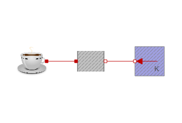
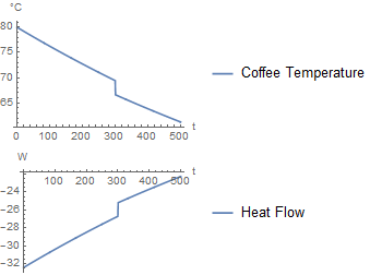
If milk is added after 300 seconds, it produces the following simulation:

Approach 2 is having a short flow of milk, instead of a instantaneous addition of milk. The benefit of this is you could create your own addition strategy. For example, you could add half of the milk at the beginning, and half after 300 seconds. Or any arbitrary strategy. For now, I focused on doing it as a 1 second pulse.
An input is added to the coffee, corresponding to the flow of milk:

The volume of the milk in the coffee is no longer a parameter but increases with the flow:
der(Vmilk) = u;
And the capacity increaces with the milk volume:
C = Ccoffee * Vcoffee * 1000 + Cmilk * Vmilk * 1000;
Adding milk will increase the enthalpy in the system, but the increased heat capacity will still cause a drop in temperature:
  T = H/C;
  der(H) = port.Q_flow + Cmilk * 1000 * u * MilkTemperature;
With H being the enthalpy.
The milk component is simply a pulse from Modelica.Blocks.Sources.Pulse that has some additional parameters.
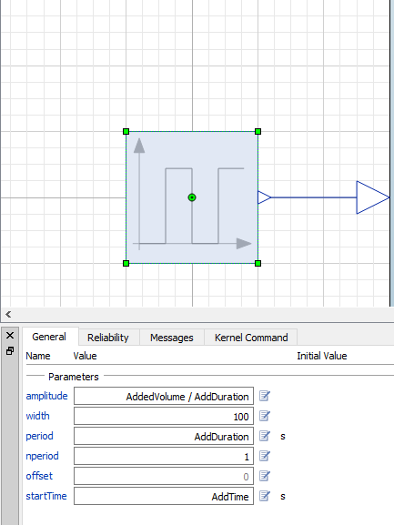
Everything taken together, we now have an additional component in the coffee cooling model:
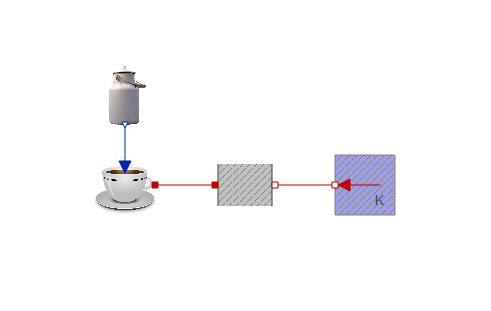
As it should, this approach gives a similar plot as the first one. The only difference is that the milk is added over a duration of 1 second. As the duration approaches zero, the two approaches would converge.
You could use this approach to fit parameters, using the methodology from the electric kettle example. I am a bit unsure if I would recommend trying fitting one of the higher order models that was suggested in the paper. With so many unknowns, you run the risk of significantly over-fitting you model. Though for a student lab, it could be a very good exercise to try and isolate each of the factors and explore them separately. I.e, cover the mug with an isolating material to avoid radiation and evaporation and take some data. Then put it in a open vacuum flask to study the evaporation without the conduction.
 Attachments: