Hi Gary!
I went through some of the models in the paper you posted. Overall, it seems like SystemModeler could be very good fit for this, allowing students to add and remove different effects and see the results. The models I show below are attached to this post. I'd love to hear more about the milk adding problem also, seems like an interesting scenario, but I am not sure I understand what the object of the students would be.
As for the paper you linked:
Experiment 1 can be described using standard components from the Modelica.Thermal.HeatTransfer package. The pot will be HeatCapacitor component, the ambient temperature will be modeled using FixedTemperature and the convection is modeled using a ThermalConductor, which follows Newtons law of cooling.
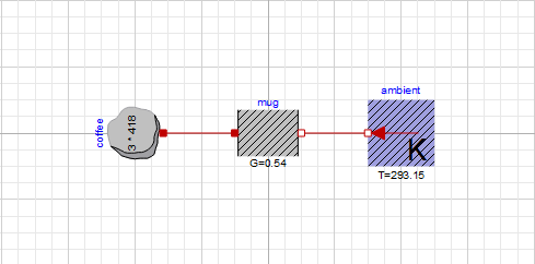
The G parameter in the ThermalConductor is equivalent to the k parameter they use. From what I could tell, the paper did not include any measurement of the heat capacitance or ambient temperature so I went with 3 dl of water and 20 degrees Celsius. However, both of these would probably need to be higher to fit their experimental data.
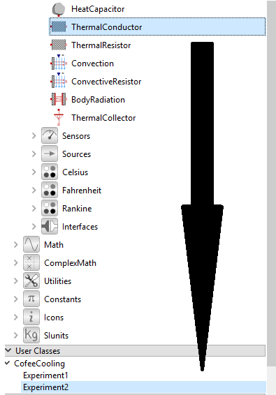
To create experiment 2 I first duplicated experiment 1 by selecting it and pressing Ctrl+D, you can also right click and select Duplicate. Experiment 2 requires a component like the ThermalConductor but one that has an exponent that causes nonlinear behaviour in the heat flow. No such component exist in the Modelica Standard Library, but we can easily create one. I created a new component to be used in experiment 2 by dragging the normal ThermalConductor into Experiment2.
And gave it a new name, "ArbitraryExponentConductor"
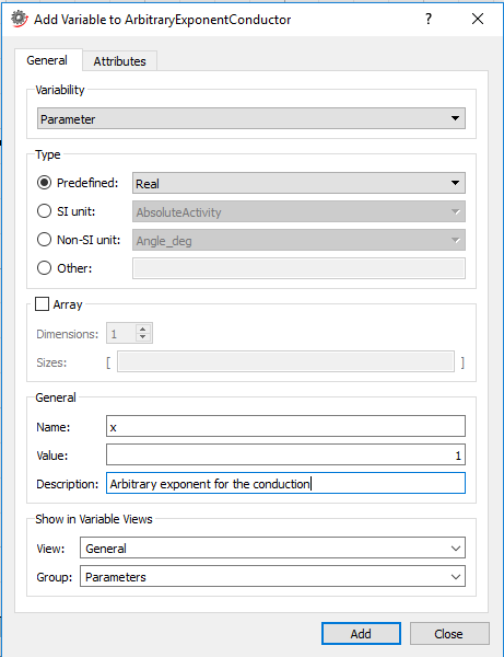
Now I had to modify it to use the exponent. After opening the new component I first added a new parameter by right clicking the parameter view and and selecting Insert > Parameter
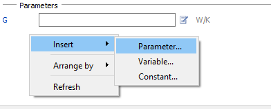
I used the name x as in the paper and used type Real.
Now I had to modify the equations so I went into the Modelica Text View (Ctrl+3) and changed the line:
Q_flow = G * dT;
to
Q_flow = G * dT ^ x;
dT corresponds to the temperature difference (tc-ts) in the paper.
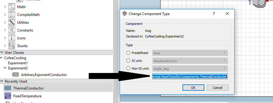
Going back into Experiment 2, I changed the normal ThermalConductor by right clicking it and selected Change Type. In the dialog, I gave the name of the new type (CofeeCooling.Experiment2.ArbitraryExponentConductor). You can also drag the component from the component browser directly into the field.
or of course, delete the component, drag the new one in and make new connections.
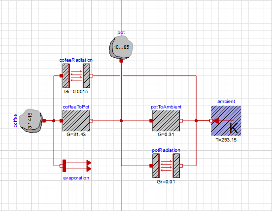
For experiment 3, you need to add a some more stuff. Start by douplicating experiment 1. Connect the ThermalConductor to a new HeatCapacitor instead of the FixtedTemperature. That heat capacitor will be the pot, while the original one will be the coffee. The first ThermalConductor then represents equation 1 in the paper, transfer of heat from coffee to the pot. Add another ThermalConductor and connect it between the pot and the FixedTemperature to represent equation 5. Also add two BodyRadiation components and connect them from each capacitor to the FixedTemperature. These will represent all the radition effects described. They are bidirectional so they represent two equations each (3,4 and 6,7). For evaporation, I created a custom component which is described by the equation
port.Q_flow = k * port.T;
Where k is the product of the P, l and v parameters described in the paper. You could add individual parameters for each of them instead, as described in the text for experiment 2.
Connect the evaporation to the coffee capacitor.
The 4:th experiment is much like the the 3:d one. I modified the evaporation component to have the equation
port.Q_flow = k * port.T ^ z;
instead. However, with the exponent they present, 3.7, the temperature will go down very fast for all but very small values of k. Without knowing what parameter they had for l, v and P, it is hard to see if that approach is sound. Do you have an idea if they published more information on the other parameters they fitted?
 Attachments:


