Message Boards Message Boards

0
|
18766 Views
|
16 Replies
|
9 Total Likes
View groups...
Share
Share this post:

Plot 2D graphs into 3D system of coordinates?

Deer Mathematica users,

There is a beautiful book by Peter Kraniauskas that made extensive use of 3d plots like the one attached to this post. enter image description here The image of having a periodic function and its different Fourier components separately is very illustrative for students. Could this plots be obtained by the Mathematica capabilities. I did try something like

data = Table[Cos[n x], {x, 0, 2 \[Pi], 0.01}, {n, 0, 5, 1}];
ListPlot3D[data, DataRange -> {{0, 10}, {0, 2 \[Pi]}}, 
 Mesh -> {13, 0}, PlotStyle -> None, PlotStyle -> Thick, 
 BoundaryStyle -> None, Boxed -> False]

enter image description here

which is still far from the desired quality.

Any ideas are welcome,

Regards

Jesús

16 Replies
Posted 5 years ago

Hi All, I have sets of FFT's. plotted 2D. I want to draw all ofthem in 3D with sampling . Other question how can I draw maximum peak points of this plot? FFTdbD is my function, I partitioned data to 36 sample. I just get FFT of each sample. I need to compare peaks or draw all FFTs in 3D.

Table[ListLinePlot[FFTdBD[data3[[All, x]], fs], Joined -> True, PlotRange -> {{0, 25}, All}, GridLines -> Automatic, Frame -> True, FrameLabel -> {"Frequency (Hz)", "a(t)(dB)"}, LabelStyle -> Directive[Black, Thin], PlotStyle -> Red], {x, 1, 36, 1}]

Thanks for your help.

POSTED BY: yigit sad

Simply write Sin[x]^n instead of Sin[n x] in the code above.

POSTED BY: Gianluca Gorni

General! Example: [Sin[x]^n] where: 0<x<3 and 1<n<5 Can we plot and show 5 -separated- "3D" graphs of sinx all in one 3D graph?

POSTED BY: Mahsa Mehrangiz

What kind of 3D forms? Spheres, cubes, cones? Each of these has its own graphics primitives, very well documented.

POSTED BY: Gianluca Gorni

Is it possible to plot 3D graphs into 3D system of coordinates?? In other words, in these algorithms we plotted 2D graphs in 3D system, how to plot their 3D forms all in one 3D system of coordinates?? I would be really appreciate if you help me.

POSTED BY: Mahsa Mehrangiz

You can use FillingStyle and PlotStyle:

Graphics3D[
 Table[Plot[Sin[n x], {x, 0, 2 Pi}, Filling -> Axis, 
     FillingStyle -> Directive[Red, Opacity[.5]], 
     PlotStyle -> Red][[1]] /. 
   GraphicsComplex[pts_, other__] :> 
    GraphicsComplex[pts /. {x_Real, y_} :> {x, n, y}, other], {n, -3, 
   3, 1}], Axes -> True, AxesStyle -> Red, AxesLabel -> {x, y, z}, 
 PlotRange -> {{-1, 7}, {-4, 4}, {-2, 2}}]
POSTED BY: Gianluca Gorni

Great! Thanks a lot

POSTED BY: Mahsa Mehrangiz

Here is an example:

Graphics3D[
 Table[Plot[Sin[n x], {x, 0, 2 Pi}, Filling -> Axis][[1]] /. 
   GraphicsComplex[pts_, other__] :> 
    GraphicsComplex[pts /. {x_Real, y_} :> {x, n, y}, other], {n, -3, 
   3, 1}],
 Axes -> True, AxesStyle -> Red, AxesLabel -> {x, y, z},
 PlotRange -> {{-1, 7}, {-4, 4}, {-2, 2}}]
POSTED BY: Gianluca Gorni

Thank You Very Much! My last question is about the filling part. In mathematica we can use fillingstyle to change the color of filling part. In this algorithm the filling part is blue. I would be really appreciate if you help me to change the color either.

POSTED BY: Mahsa Mehrangiz

Hello, I use the algorithm which has been written by "Gianluca Gorni, University of Udine " but I have 3 questions: 1. how to change the axis color? 2. how to show the range of axis? 3. how to use axis labels?

I would be appreciate if you answer me.

POSTED BY: Mahsa Mehrangiz

Hi Jesus,

Your picture is an isometric line drawing. All such images are easy to draw by constructing the three dimensional curves, choosing the view vectors, and projecting into the plane. If you get more detailed, the main difficulty becomes the ordering and stacking along the axis of projection. I think it's advantageous to use Graphics as opposed to Graphics3D because the output of Graphics is a scalable vector, seems to be more reliable for including in papers. I've already given a few examples in a recent topic:

Plotting the Contours of Deformed Hyperspheres

Here's another example more along the lines of what you are looking for:

Function Definitions

Amp = Normalize[(-1)^# Exp[-#] & /@ Range[4]];
fs = Times[Cos[k x] /. k -> (# 2 Pi) & /@ Range[4], Amp];
F = Total[fs];
f0 = -(F /. x -> 0);
F2 = f0 + F;

View Settings

ViewV = Normalize@ {1, -1, 1};
xOrtho = Normalize@{1, 1, 0};
yOrtho = Normalize@Cross[ViewV, xOrtho];
Projector = {xOrtho, yOrtho};
colors = Partition[{Red, Orange, Yellow, Green, Blue}, 2, 1];
intRatio = {25, 9, 3, 2};

Curve to Points

GetLine[fx_, xm_, xp_] :=  Cases[Plot[fx, {x, xm, xp}, PlotRange -> All], Line[_], Infinity]
GetLine[fx_, xm_, xp_, n_, m_] :=  Join[#, {{#[[-1, 1]], 0}, {#[[1, 1]], 0}} ] & /@ Partition[
With[{nMax = Max[Flatten[Partition[Range[0, n], m, m - 1]]]},
N[Map[{(xm + # (xp - xm)), fx /. x -> (xm + # (xp - xm))} &, 
Range[0, nMax - 1]/(nMax - 1)]]  ], m - 1, m]    
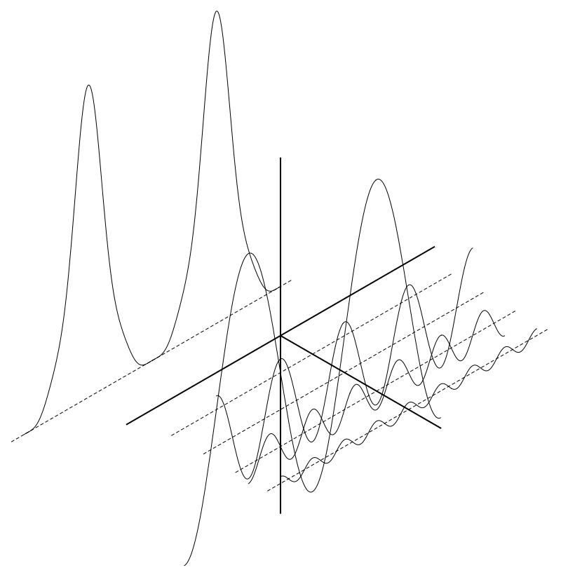
Simple Output

Graphics[Join[
MapThread[{{Dashed, 
Line[Projector.# & /@ {{#2/4, -1.1, 0}, {#2/4, 1.1, 0}}]},
GetLine[#1, -1, 1] /. {y_, z_} :> Projector.{#2/4, y, z}} &,
{fs, Range[4]}],
{{Thick, Line[Projector.# & /@ {{0, 0, 0}, {5/4, 0, 0}}], 
Line[Projector.# & /@ {{0, 0, -1.2}, {0, 0, 1.2}}],
Line[Projector.# & /@ {{0, -1.2, 0}, {0, 1.2, 0}}]}, {
{Dashed, Line[Projector.# & /@ {{-1, -1.1, -f0}, {-1, 1.1, -f0}}]},
GetLine[F, -1, 1] /. {y_, z_} :> Projector.{-1, y, z}
}}], ImageSize -> 800]
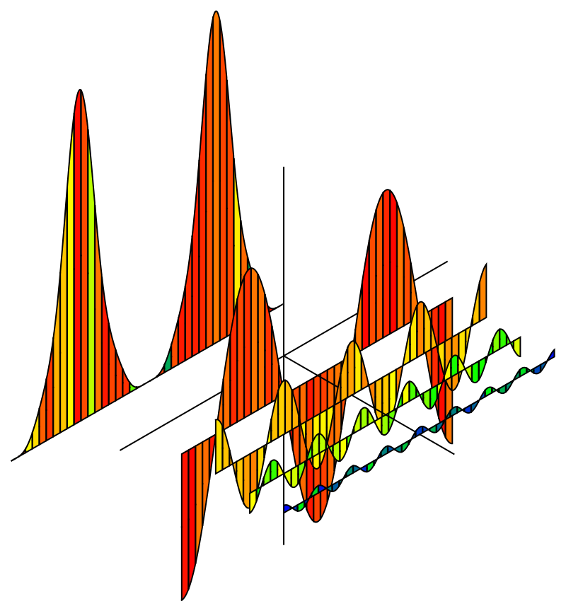
BWLineDrawing

Color Line Drawing

g1 = Graphics[{EdgeForm[Thick], MapThread[{#1, #2} &,
{RandomSample[
Flatten[MapThread[
Table[Blend[#1, RandomReal[{0, 1}]], {#2}] &, {colors, 
intRatio}]]],
Polygon[# /. {y_, z_} :> Projector.{-1, y, z - f0}] & /@ 
GetLine[F2, -1, 1, 2000, 50]}]}];

Show[ g1, Graphics[{Thick,
Line[Projector.# & /@ {{0, 0, 0}, {1/4, 0, 0}}],
Line[Projector.# & /@ {{0, -1.2, 0}, {0, 1.2, 0}}],
Line[Projector.# & /@ {{0, 0, -1.2}, {0, 0, 1.2}}]}],
MapThread[DrawPart, {fs, Range[4]/4, Table[1/4, {4}], colors}],  
ImageSize -> 800]

ColorFourier

POSTED BY: Brad Klee

Brad

That is just great. Thanks.

It seems that the graphic capabilities of mathematica are endless.

I will be working with ideas obtained here.

regards

Jesus

How about this:

Graphics3D[
 Table[Plot[Sin[n x], {x, 0, 2 Pi}, Filling -> Axis][[1]] /. 
   GraphicsComplex[pts_, other__] :> 
    GraphicsComplex[pts /. {x_Real, y_} :> {x, n, y}, other],
  {n, -3, 3, 1}]]

enter image description here

It makes 2D sin plots with Filling, and then lifts them into 3D.

POSTED BY: Gianluca Gorni

Great! It is a lot better.

Regards

Jesus

Gianluca

I think was a very good One-Liner! Thanks again.

Jesus

Hello, I used the algorithm which has been written by "Gianluca Gorni, University of Udine " but I have 2 questions: 1. how to change the axis colors? 2. how to show the range of axis?

I would be appreciate if you answer me.

POSTED BY: Mahsa Mehrangiz
Reply to this discussion
Community posts can be styled and formatted using the Markdown syntax.
Reply Preview
Attachments
Remove
or Discard

Group Abstract Group Abstract