Message Boards Message Boards

29
|
103671 Views
|
22 Replies
|
119 Total Likes
View groups...
Share
Share this post:

[CALL] Most common pitfalls for beginners of Wolfram Language

Wolfram Language (WL) is a powerful multi-paradigm programing language. There is a set of common mistakes that repeatedly tend to entrap new users. This is a call to describe such mistakes building a "black-listing" guide for novice coders. Please consider contributing. I suggest following simple rules (with gratitude adapted from a similar effort):

  • One topic per answer

  • Focus on non-advanced uses (it is intended to be useful for beginners and as a question closing reference)

  • Include a self explanatory title in header style (example: "# Basic built-in function syntax"; see syntax guide )

  • Explain the symptoms, the mechanism behind the scenes and all possible causes and solutions you can think of. Be sure to include a beginner's level explanation (and a more advance one too, if you can)

Please, use "Reply" to a specific comment for structured clarity of nested comments.


Table of Contents

POSTED BY: Vitaliy Kaurov
22 Replies
Posted 3 years ago

Keyboard combinations and keyboard mistakes. I'm a longtime Mathematica user but am surprised by the recent inadvertent results when trying to add comments to input. The second line below, the red square, is particularly problematic. It appears at the beginning of the input line and will change the properties of what is usually a variable and assignment operator (set). If it occurs with a variable that is subscripted, I have to reboot Mathematica; undo, Clear[], ClearAll[] will not fix whatever that red square does to my subscripted variables. The freeform input symbol shown is easy to search for (orange box with equals sign), but not so with the red box and other mistakes shown....

Wolfram Notebook

POSTED BY: Mark Bourland
Posted 3 years ago

Differences between "Equal" and "SameQ"


There are different ways of comparing two elements or more, the first one is less strict: using Equal (==); the second one, is more strict: using SameQ (===).

Let's take a look at the documentation page for Equal:
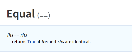
Equal Documentation Page

And now, the documentation page for SameQ...

SameQ Documentation Page

This alone doesn't tell much, but how exactly these two operators (== and ===) are different? The difference lies in their individual strictness.

If you want to compare numbers AND their types, use SameQ, if you want less strict comparisons, use Equal.
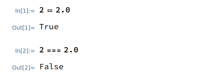
Equals vs SameQ

Sometimes, Equal outputs a symbolic equation, and that can be bad sometimes, if you want to ALWAYS output a boolean value, use SameQ.
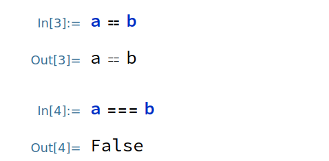
Equal Symbolic vs SameQ Boolean

WARNING: SameQ has a higher precedence as an operator. If you want to replace values, replace the values while holding the operation.
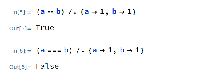
SameQ precedes Equal

POSTED BY: Pedro Cabral

Don't perform operations on whole arrays by indexing individual elements....

Horrible:
output = ConstantArray[0, Length[data]]; 
For[j = 1, j <= Length[data], j++, output[[j]] = Sin[data[[j]]]];
output

Bad:
Table[Sin[data[[j]]], {j, 1, Length[data]}]

Nice:
Map[Sin, data]

And if the operation is Listable... Best: Sin[data]

POSTED BY: Jon McLoone

If i would get a euro for every time I see horrible/bad approach…

POSTED BY: Sander Huisman

Subscripted variables are a pain...use [i] indexing instead.

POSTED BY: Yaroslav Bulatov

Properties & Relations of constraining a locator

Since the example of constraining a (interactive, or, editable) point or locator to the edge of the unit circle appears over and over again in different yet similar teaching contexts, it can become confusing for the beginner to discern all the coding variations by heart and know which one to use in a given active coding situation. In order to constrain a locator (or point or plot tracker/tracer or alike) key functions can be Locator, LocatorPane, Dynamic, DynamicModule, Manipulate, TrackingFunction, Slider2D, but not all of them at the same time. It depends on what you want and what you start with.

In the end it all boils down to the exploitation of the optional 2nd argument of Dynamic which must be a function (or a list of functions); typically the function is a pure function func[val, expr] processing the "mouse position" (val) and the dynamic expression expr (usually just a single dynamic variable u).

The attached short notebook tries to give a helpful overview of all seven (common) variations for reference and easy comparison.

Also check out the Monday morning quiz testing your beginner's Wolfram L vocabulary!

Attachments:
POSTED BY: Raspi Rascal
Posted 8 years ago

Import and "CurrencyTokens"

Perhaps not 'common' but I was bitten by it twice until I made it 'my' default for data import. I assume for some legacy reason the stripping of currency symbols is the default behavior of the Import[] function. Seems an odd default behavior to me and worse the default behavior is not pointed out as boldly as I think it should be in the documentation.

Import[   , "CurrencyTokens" -> None]

Incorrect Import

Correct Import

POSTED BY: David Proffer

Numerical vs Symbolic -- What to do when plots are blank (and other strange errors)

The plotting functions require numerical inputs. This sounds obvious but most people have trouble debugging plots that come out empty. When something does not plot, the first thing to do is to evaluate the expression and look for undefined variables or typos.

Consider the following:

A = 12;
b = 3;
expr = a* b sin[theta];
Plot[expr, {theta, 0, 10}]

which yields a less than informative plot:

enter image description here

The best approach is to take the plot argument and evaluate it at a point somewhere in the plot range and see that it is numerical. It is often a good idea to evaluate it at the two extremes and the middle to make sure it is numerical everywhere.

expr /. theta -> 0
expr /. theta -> 5
expr /. theta -> 10

to get

 (* 3 a sin[0] 
3 a sin[5] 
3 a sin[10] *)

It becomes clear that the a is undefined and that sin does not evaluate (because of the lower case 's')

POSTED BY: Neil Singer

Case sensitivity and typos

I am far from a novice user, but I make a lot of typing mistakes, so case sensitivity catches me often...especially on properties and names in WDF, etc.

This command gets an error

ResourceData["On the origin of Species"]

This command gets the data

ResourceData["On the Origin of Species"]

This command gets an error...also I find the error message to be somewhat opaque

DateObject[{2016, 8, 4}, "week"]

This command evaluates the object

DateObject[{2016, 8, 4}, "Week"]
POSTED BY: Aeyoss Antelope

Consider Reap/Sow Instead of AppendTo

When using the output of a program to build large lists, a combination of Reap and Sow is often cited as the most efficient (computationally speaking) approach. Put simply, AppendTo trades speed in favour of flexibility by creating a copy of the original list when called. Indeed, Reap/Sow is also point 7 of 10 Tips For Writing Fast Mathematica Code.

I remember first seeing Reap/Sow as a beginner and feeling like it was an 'advanced' feature for other users. Instead I fell into the pattern of defining an empty list and using AppendTo which in hindsight was a beginner's mistake I frequently made by the justification given above.

The example from the link above says it best:

In[7]:= data = {}; 
 Do[AppendTo[data, RandomReal[x]], {x, 0, 40000}]; // AbsoluteTiming

Out[7]= {11.6127, Null}

In[8]:= data = 
   Reap[Do[Sow[RandomReal[x]], {x, 0, 40000}]][[2]]; // AbsoluteTiming

Out[8]= {0.164533, Null}

This is one small change which will Reap large benefits for any beginner.

POSTED BY: Benjamin Goodman

Alternatives to Reap/Sow

1. I would like to mention Table[] in addition. In complicated situations, Reap and Sow maybe be a better alternative, but I've seen quite a bit of beginner's code that looks just like the Do-AppendTo loop above. In that particular case, Table[] is superior both in speed and legibility. It's about 20 times faster than the Reap version:

data = Table[RandomReal[x], {x, 0, 40000}];

(Asides: In some use cases, Map may be an even better choice. Also, many functions are "vectorized" or have special cases for efficiently constructing arrays; for instance, RandomReal[1, 40001] * Range[0., 40000.] produces nearly the same data 150 times faster than Reap, the maximum relative error being less than 10^-12 -- learning to think computationally in terms of arrays can speed up code significantly.)

2. Let me also add linked lists as an alternative (see also this answer by Leonid Shifrin). It is 5-10% faster than Reap & Sow.

data = {};
Do[data = {data, RandomReal[x]}, {x, 0, 40000}];
data = Flatten@data;

If the data is an multidimensional array, then we can structure the flattening operation by using a special head.

Block[{ll},    (* not necessary if  ll  is undefined *)
 data = ll[];
 Do[data = ll[data, RandomReal[x, 2]], {x, 0, 40000}];
 data = List @@ Flatten[data, Infinity, ll];
 ]

Example timing:

SeedRandom[0];    (* for reproducible randomness *)
data = Reap[Do[Sow[RandomReal[x, 2]], {x, 0, 40000}]][[2, 1]]; // AbsoluteTiming
(*  {0.097571, Null}  *)

SeedRandom[0];    (* for reproducible randomness *)
dataLL = ll[];
(Do[dataLL = ll[dataLL, RandomReal[x, 2]], {x, 0, 40000}]; 
   dataLL = List @@ Flatten[dataLL, Infinity, ll]); // AbsoluteTiming
(*  {0.08676, Null}  *)

data == dataLL
(*  True  *)
POSTED BY: Michael Rogers

What does @#(%=<[!} et cetera mean?

Mathematica has a very extensive set of characters used as its syntax. I will try to list most (all?) of them here.

Non-standard characters

If the symbol appears to be a non-standard character one can wrap the symbol in quotes and perform FullForm on it to get the name of the symbol. Example:

enter image description here

gives:

"\[Function]"

Brackets

These syntax elements all appear in pairs:

  • (...) Circumfix. Used to group expressions such that it has higher precedence, not used to enclose arguments of a function
  • {...} List doc. Circumfix. Used to describe lists of any depth, e.g.: {a,b,...}. Known as arrays, vectors, matrices, tensors, in other languages
  • [...] Circumfix. Used to enclose arguments of a function, e.g.: f[a]
  • [[...]] Part doc. Post/circumfix. a[[b]] = Part[a,b]. Used to extract parts of an expression. Can also be typeset as a single character: \[LeftDoubleBracket] and \[RightDoubleBracket], and can also be typeset as a subscript
  • <|...|> Association doc. Circumfix. Used to describe a list of key-value pairs. Known as associative arrays, dictionaries, hashmaps. Can also be typeset as a single character: \[LeftAssociation] and \[RightAssociation].
  • (*...*) Circumfix. Used for making comments in code, can be anywhere in the code except inside strings, then it will be taken literal.
  • <*...*> TemplateExpression doc. Circumfix. Expression inside a string template.
  • \[LeftFloor]...\[RightFloor] Floor doc. Circumfix. Mathematical Floor function. \[LeftFloor]a\[RightFloor] = Floor[a]. Can be typeset using \[LeftFloor] and \[RightFloor].
  • \[LeftCeiling]...\[RightCeiling] Ceiling doc. Circumfix. Mathematical Ceiling function. \[LeftCeiling]a\[RightCeiling] = Ceiling[a]. Can be typeset using \[LeftCeiling] and \[RightCeiling].

Applying functions

  • @ doc. Infix. Used to apply a function to a single argument: f@x = f[x] (related to Prefix doc)
  • // doc. Infix. Used to apply a function to a single argument: x // f = f[x] (related to Postfix doc)
  • ~ Infix. Works on two arguments: a ~ f ~ b = f[a,b] (related to Infix doc)
  • @* Composition doc. Infix. f@*g = Composition[f,g] Used to compose two or more functions. @* is the infix operator form of Composition
  • /* RightComposition doc. Infix. f/*g = RightComposition[f,g] Used to compose two or more functions. /* in the infix operator form of RightComposition
  • /@ Map doc. Infix. f/@ a = Map[f,a] Used to apply a function to all elements of a
  • //@ MapAll doc. Infix. f//@ a = MapAll[f,a] Used to apply a function to every subexpression of a
  • @@ Apply doc. Infix. f @@ a = Apply[f,a] Used to replace the head of a by f
  • @@@ Apply doc. Infix. f @@@ a = Apply[f,a,{1}] Used to replace the heads at level 1 of a by f.

Pure function, slots, and slot sequences

  • & Function doc. Used to define a pure function where the arguments are given by #1 (short: #), #2, #3, et cetera. Also known as lambda function, anonymous functions, function literal, lambda abstraction...
  • # Slot doc. represents the first argument supplied to a pure function
  • #1, #2, #n Slot doc. represents the nth argument supplied to a pure function
  • #0 Slot doc. represents the pure function itself.
  • #name Slot doc. represents the value associated with the key name in an association in the first argument
  • ## SlotSequence doc. represents a sequence of all the arguments
  • ##n SlotSequence doc. represents a sequence of arguments starting from the nth
  • \[Function] Function doc. Infix operator of Function. x \[Function] body = Function[x,body]
  • |-> Function doc. Infix operator of Function with names variable. x |-> body = Function[x,body]

Assignments

  • = Set doc. Infix. a=b = Set[a,b]
  • := SetDelayed doc. Infix. a:=b = SetDelayed[a,b]
  • =. Unset doc. Postfix. a=. = Unset[a]
  • ^= UpSet doc. Infix. a[b]^=c = Upset[a[b],c]
  • ^:= UpsetDelayed doc. Infix. a[b]^:=c = UpSetDelayed[a[b], c]
  • /: = TagSet doc. Compound infix. a /: b[a] = c = TagSet[a, b[a], c]
  • /: := TagSetDelayed doc. Compound infix. a /: b[a] := c = TagSetDelayed[a, b[a], c]
  • /: =. TagUnset doc. Compound infix. a /: b[a] =. = TagUnset[a, b[a]]
  • += AddTo doc. Infix. a+=b = AddTo[a, b] Adds b to a and stores the value in a.
  • -= SubtractFrom doc. Infix. a-=b = SubtractFrom[a, b] Subtracts b from a and stores the value in a.
  • *= TimesBy doc. Infix. a*=b = TimesBy[a, b] Multiplies a by b and stores the value in a.
  • /= DivideBy doc. Infix. a/=b = DivideBy[a,b] Divides a by b and stores the value in a.
  • //= ApplyTo doc. Infix. a//=f = ApplyTo[a,f]. Applies function f to a and stores the value in a.
  • ++ used as a prefix operator is PreIncrement doc. ++a = PreIncrement[a] Adds 1 to a and stores the value in a, returns the new a
  • ++ used as a postfix operator is Increment doc. a++ = Increment[a] Adds 1 to a and stores the value in a, returns the old a
  • -- used as a prefix operator is PreDecrement doc. --a = PreDecrement[a] Subtracts 1 from a and stores the value in a, returns the new a
  • -- used as a postfix operator is Decrement doc. a-- = Decrement[a] Subtracts 1 from a and stores the value in a, returns the old a

Number related

  • *^ Infix. Equivalent to *10^ sometimes 'e' in other languages. 3*^4 = 30000
  • ` related to Precision doc. Postfix. Define number to be a machine precision number. It denotes context when it is written between symbols. Also appears in pairs inside strings for TemplateSlot doc where they denote an argument
  • `n related to Precision doc. Infix. Defines number to have precision n. It denotes context when it is written between symbols
  • ``n related to Accuracy doc. Infix. Supposed to be written between 2 numbers. Defines number to have accuracy n
  • ^^ related to BaseForm doc. Infix. 3^^1212 represents 1212 written in base 3. Up to base 36 can be specified in this notation (using letters a through z, in either lower of upper case, to denote 10 through 35). Use FromDigits doc for higher bases. Base conversion is done using IntegerDigits doc or RealDigits doc
  • \[ImplicitPlus] ImplicitPlus doc. Infix. An invisible character used for e.g. fractions: 5\[ImplicitPlus](3/4) = Plus[5,3/4] = 23/4 where 3/4 is then typed as a fraction

Relational operators

  • == Equal doc. Infix. a==b = Equal[a,b]. Used to test if a and b are equal. Also used to define an equation
  • \[Equal] Equal doc. Infix. a==b = Equal[a,b]. Used to test if a and b are equal
  • != UnEqual doc. Infix a!=b = UnEqual[a,b]. Used to test if a and b are not equal
  • ? UnEqual doc. Infix a!=b = UnEqual[a,b]. Used to test if a and b are not equal
  • > Greater doc. Infix. a>b = Greater[a,b]. Used to test if a is greater than b
  • < Less doc. Infix. a<b = Less[a,b]. Used to test if a is less than b
  • >= GreaterEqual doc. Infix. a>=b = GreaterEqual[a,b]. Used to test if a is great than or equal to b
  • <= LessEqual doc. Infix. a<=b = LessEqual[a,b]. Used to test if a is less than or equal to b
  • === SameQ doc. Infix. a===b = SameQ[a,b]. Used to test if a and b are identical
  • =!= UnsameQ doc. Infix. a=!=b = UnsameQ[a,b]. Used to test if a and b are not identical

Note: All the above operator can remain unevaluated, except for SameQ and UnsameQ, these always evaluate to either True or False. Even when a or b is symbolic. All operator can be used multiple times in a row e.g.: a == b == c (all have to be equal) or a > b > c (strictly decreasing numbers) or a != b != c (all unequal). The functions have arbitrary arity, e.g. Equal[] = True.

  • \[Element] Element doc. Infix. a \[Element] b = Element[a,b]. Asserts that a is an element of b

Logical operators

  • &&, \[And] And doc. Infix. Logical And operator. a && b = a \[And] b = And[a,b] Executes in order and has lazy evaluation
  • ||, \[Or] Or doc. Infix. Logical Or operator. a || b = a \[Or] b = Or[a,b] Executes in order and has lazy evaluation
  • \[Nand] Nand doc. Infix. Logical Nand operator a \[Nand] b = Nand[a,b] Executes in order and has lazy evaluation
  • \[Nor] Nor doc. Infix. Logical Nor operator a \[Nor] b = Nor[a,b] Executes in order and has lazy evaluation
  • ! Not doc. Prefix. Logical negation !a = Not[a]. Not to be confused with Factorial doc (postfix operator)
  • ¬ Not doc. Prefix. Logical negation ¬a = Not[a].
  • \[Xor] Xor doc. Infix. Logical Xor operator a \[Xor] b = Xor[a,b]
  • \[Implies] Implies doc. Infix. Logical implication. a \[Implies] b = Implied[a,b]
  • \[Equivalent] Equivalent doc. Infix. Logical equivalence testing. a \[Equivalent] b = Equivalent[a,b]

Note: And, Or, Nand, Nor, and Xor have arbitrary arity.

Patterns and rules

  • _ Blank doc. Prefix. _ = Blank[]
  • _a Blank doc. Prefix. _a = Blank[a]
  • __ BlankSequence doc. Prefix. __ = BlankSequence[]
  • __a BlankSequence doc. Prefix. __a = BlankSequence[a]
  • ___ BlankNullSequence doc. Prefix. ___ = BlankNullSequence[]
  • ___a BlankNullSequence doc. Prefix. ___a = BlankNullSequence[a]
  • a_ Pattern doc. Postfix/infix. a_ = Pattern[a, Blank[]]
  • a:_ Pattern doc. Postfix/infix. a:_ = Pattern[a, Blank[]]
  • a__ Pattern doc. Postfix/infix. a__ = Pattern[a, BlankSequence[]]
  • a:__ Pattern doc. Postfix/infix. a:__ = Pattern[a, BlankSequence[]]
  • a___ Pattern doc. Postfix/infix. a__ = Pattern[a, BlankNullSequence[]]
  • a:___ Pattern doc. Postfix/infix. a:__ = Pattern[a, BlankNullSequence[]]
  • _. Optional doc. Postfix. _. = Optional[Blank[]] also related to Default doc
  • _:a Optional doc. Postfix. _:a = Optional[Blank[],a] also related to Default doc
  • __. Optional doc. Postfix. __. = Optional[BlankSequence[]] also related to Default doc
  • __:a Optional doc. Postfix. __:a = Optional[BlankSequence[],a] also related to Default doc
  • ___. Optional doc. Postfix. ___. = Optional[BlankNullSequence[]] also related to Default doc
  • ___:a Optional doc. Postfix. ___:a = Optional[BlankNullSequence[],a] also related to Default doc
  • /; Condition doc. Infix. a /; b = Condition[a, b]
  • ? PatternTest doc. Infix. a ? b = PatternTest[a,b]
  • -> Rule doc. Infix. a -> b = Rule[a,b]
  • \[Rule] Rule doc. Infix. a \[Rule] b = Rule[a,b]
  • :> RuleDelayed doc. Infix. a :> b = RuleDelayed[a,b]
  • \[RuleDelayed] RuleDelayed doc. Infix. a \[RuleDelayed] b = RuleDelayed[a,b]
  • /. ReplaceAll doc. Infix. a /. b = ReplaceAll[a, b]
  • //. ReplaceRepeated doc. Infix. a //. b = ReplaceRepeated[a,b]
  • .. Repeated doc. Postfix. a.. = Repeated[a]
  • ... RepeatedNull doc. Postfix. a... = RepeatedNull[a]
  • | Alternatives doc. Infix. a | b = Alternatives[a, b]. Not to be confused with || Or doc

String related

  • <> StringJoin doc. Infix. a<>b = StringJoin[a,b]
  • ~~ StringExpression doc. Infix. a~~b = StringExpression[a,b]

Note: both have arbitrary arity.

Graph related

  • <-> UndirectedEdge doc. Infix. a<->b = UndirectedEdge[a,b]
  • \[UndirectedEdge] UndirectedEdge doc. Infix. a\[UndirectedEdge]b = UndirectedEdge[a,b]
  • \[DirectedEdge] DirectedEdge doc. Infix. a\[DirectedEdge]b = DirectedEdge[a,b]

Other

  • \[Application] Application doc a\[Application]b Performs Application[a,b].
  • . Dot doc a.b Performs the dot product of a and b
  • , Used to separate arguments in a function call, e.g.: f[a,b]
  • % Out doc. % = Out[$Line - 1] = Out[]. Gives the last result generated
  • %% Out doc. %% = Out[-2]. Gives the penultimate result
  • %..% (k repetitions of %) Out doc. %...% = Out[-k]. Gives the k-th last result
  • %n Out doc. Gives the result of line n
  • \[PartialD] D doc. Postfix. Use in combination with a subscript to denote a partial derivate
  • \[DifferentialD] Integrate doc. Compound match fix. \[Integral]a\[DifferentialD]b = Integrate[f,b]
  • ! as a postfix operator means Factorial doc a! = Factorial[a]. Mathematical factorial function
  • !! as a postfix operator means Factorial2 doc a!! = Factorial2[a]. Mathematical double factorial function
  • ; CompoundExpression doc. Infix. a=1;a=2 = CompoundExpression[a=1,b=2] Though it might look like a postfix operator, it is not: a=1;a=2; = CompoundExpression[a=1,b=2,Null]
  • ;; Span doc. Infix. a ;; b = Span[a,b] and a ;; b ;; c= Span[a,b,c] Note that more than 2 infix operator in a row will give (most likely) unexpected results
  • :: MessageName doc. Infix. a::b = MessageName[a,b]
  • ? Information doc. Prefix. ?a = Information[f, LongForm -> False]. Print some information about symbol a
  • ?? Information doc. Prefix. ??a = Information[f]. Print information about symbol a
  • << Get doc. Prefix. << a = Get["a"]. Reads in file a, evaluating each expression in it and returning the last one. Not to be confused with left bit shift operators in other languages (BitShiftLeft doc)
  • >> Putt doc. Infix. a >> b = Put[a,b]. Write a to file b. Not to be confused with right bit shift operators in other languages (BitShiftRight doc)
  • >>> PutAppend doc. Infix. a >>> b = PutAppend[a,b]. Appends a to file b.

In case some symbol(s) is(are) missing, let me know!

POSTED BY: Sander Huisman

New in 12.2, ApplyTo x//=f

It's included on the Input Operator Forms webpage.

POSTED BY: Raspi Rascal

Thanks, had added a previous version of ApplyTo, now fixed, and also added [Application]. (https://reference.wolfram.com/language/ref/Application.html)

POSTED BY: Sander Huisman

see "x|->f — new syntax for Function with named variables"

btw your post is the only bookmark I am keeping from this community site.

POSTED BY: Raspi Rascal

Also added this explicitly. thanks!

POSTED BY: Sander Huisman

For some reason the following code is not working for me: ?5.5?=Missing["UnknownSymbol", "5.5?"] Has the floor function syntax been updated?

POSTED BY: Peter Burbery
Posted 3 years ago

Not sure how you are entering the left and right floor brackets but that is the problem,

\[LeftFloor]5.5\[RightFloor]
(* 5 *)

To enter from the keyboard esclfesc and escrfesc where esc is escape.

POSTED BY: Rohit Namjoshi

The forum screwed up some of the symbols and replaced them with ?. Now fixed.

POSTED BY: Sander Huisman

Sorting numerical data and the behavior of Sort

Mathematica has various ways of sorting data. Most commonly one wants to sort numbers. The command Sort can be used to do so:

Sort[{4, 2, 8, 1}]

returns:

{1, 2, 4, 8}

all very well. However, if one has symbolic answers, Sort might not do what you expect:

data3 = Sin[Range[10]]
data3 // N
Sort[data3]

gives:

{Sin[1],Sin[2],Sin[3],Sin[4],Sin[5]}
{0.841471,0.909297,0.14112,-0.756802,-0.958924}
{Sin[1],Sin[2],Sin[3],Sin[4],Sin[5]}

It looks like if Sort did not do anything! What is happening here? Well, Sort puts things in canonical order and decides whether they are ordered correctly using the default function Order (which works basically the same as OrderedQ):

OrderedQ[1,2]  (* True, they are ordered *)
OrderedQ[2,1]  (* False; they are not ordered *)
OrderedQ[Sin[2], Sin[3]]    (* True, they are ordered! *)

That might be a bit unexpected. Sort will only look at the structure, and then 2 comes before 3. If we want to explicitly sort by numerical value (rather than canonical order) one needs to specify this:

data3 = Sin[Range[5]]
data3 // N
Sort[data3, Less]  (* prior to V11.1 *)
N[%]
Sort[data3, NumericalOrder]   (* V11.1 and up *)
N[%]

One can do this in the above two ways (using NumericalOrder rather than Order) or using the function Less which will evaluate the number numerically and then compare them. Since Version 11.1 there is also a new function called NumericalSort which just does that:

data3 = Sin[Range[5]]
data3 // N
NumericalSort[data3]
N[%]

Now that we know why Sort sometimes gives unexpected results, and that we have found alternate ordering functions, we find that this is generally not fast.

data = RandomReal[1, 10^6];
AbsoluteTiming[Sort[data, Less];]

It takes several seconds (5.3 seconds on my laptop) to sort a million numbers! Ok, what's going on here? The problem is that Sort with a second argument does pair-wise comparisons, such that the algorithm scales very poorly. If the problem can be re-stated such that each element in a list gets a numerical value which can be sorted using the default ordering function (Order), then this is much faster. We can then improve the performance considerably by using SortBy and a second argument:

AbsoluteTiming[SortBy[data, N];]

or equivalently in this case (we already have approximate numbers so N is not necessary):

AbsoluteTiming[SortBy[data, Identity];]

which only takes 0.17 seconds on my laptop. Since we have approximate numbers, Sort itself works correctly and is fast as well:

AbsoluteTiming[Sort[data];]

Takes 0.16 seconds on my laptop.

Summary

  • If one only has pure numbers (1337, 1.337 et cetera) use Sort (or from version 11.1 on use NumericalSort).

  • If one has numbers but in some kind of symbolic form (Sin[3], Sqrt[5], Pi, E, Exp[2], 10 Degree, Quantity[Sqrt[..],...] or ...) use NumericalSort (or SortBy[... , N] for versions prior to 11.1).

  • If your problem is not one of those, then check if the problem can be recast in one where a single function gives a 'value' to each element that then can be sorted efficiently, if that is possible use SortBy with the correct second argument

Compare the following two examples:

SortBy[{"abc","ab","e","cd","efg"},StringLength]
Sort[{"abc","ab","e","cd","efg"},StringLength[#1]<=StringLength[#2]&]

Give the same result but the first one is generally much faster.

  • If such a rephrasing of the problem is not possible use the general Sort with appropriate ordering function.

Final words

Much more can be said about Sort (like the ordering of Sort for a mix of strings, symbols, and numbers). Feel free to comment on this post for additional things to consider when sorting...

POSTED BY: Sander Huisman

Learn how to use the Documentation Center effectively

Mathematica comes with the most comprehensive documentation I have ever seen in a software product. This documentation contains

  • reference pages for every Mathematica function
  • tutorials for various topics, which show you step by step how to achieve something
  • guide pages to give you an overview of functions about a specific topic
  • a categorised function navigator, to help you find appropriate guide pages and reference pages.
  • finally, the complete interactive Mathematica book

You can always open the Documentation Center by pressing F1. When the cursor (the I-beam) is anywhere near a function, then the help page of this function is opened. E.g. when your cursor is anywhere at the position where the dots are in .I.n.t.e.g.r.a.t.e., you will be directed to the help page of Integrate.

Reference pages:

A reference page is a help page which is dedicated to exactly one Mathematica function (or symbol). In the image below you see the reference page for the Sin function. Usually, some of the sections are open, but here I closed them so you see all parts at once.

enter image description here

  • In blue, you see the usage. It gives you instantly information about how many arguments the function expects. Often there is more than one usage. Additionally, a short description is given.
  • The Details section gives you further information about Options, behavioural details and things which are important to note. In general, this section is only important in a more advanced state.
  • In some cases, extra information is provided on the mathematical Background of the function explaining the depths of the method, its relation to other functions and its limitations (for example FindHamiltonianCycle).
  • The Examples section is the most important, because there you have a lot of examples, showing everything starting from simple use cases to very advanced things. Study this section carefully!
  • See Also gives you a list of functions which are related. Very helpful, when a function does not exactly what you want, because most probably you find help in the referenced pages.
  • Tutorials shows you tutorials which are related to the function. In the case of Sin it is e.g. the Elementary Transcendental Functions tutorial.
  • Related Guides gives you a list of related guide pages.
  • Related Links references to material in the web: Demonstrations, MathWorld pages, etc.

In general, my recommendation for viewing a help page is the following:

  1. Study the usage carefully
  2. Look up basic examples. If you don't find what you need, look up all examples
  3. Read the Details

And of course if you like the how-to style, you should read the referenced tutorials.

Guide pages:

Guide pages collect all functions which belong to a certain topic and they are an excellent resource when you try to find a function you do not know yet.

enter image description here

The guide page itself is often divided into several subsections collecting similar functions. In the image above, for instance, the Trigonometric Functions. Furthermore, you can find links to tutorials, etc. when you open the Learning Resources tab. At the end of each guide page, you will find references to related guide pages.

Final notes:

  • Since the complete documentation consists of usual Mathematica notebooks, all calculations and examples can be tested inside the help pages. Of course, you cannot destroy the documentation, because everything is reset when you close a help page.

  • You can always search the documentation by typing into the search bar on top of the Documentation Center:

    enter image description here

  • When coming from a different programming language, and you are not sure that a certain Mathematica function is equivalent to what you are used to, be sure to check the Properties & Relations section in the reference page to get ideas on what other functions could be relevant for your case.


Please find the original discussion here.

POSTED BY: Patrick Scheibe

Basic syntax of built-in functions

  • All built-in functions start from capital letters and are in CamelCase for compound names. Users of many other programming languages might miss this as they are used to different conventions. Examples: Plot, ListPlot, FindSpanningTree, etc.

  • Arguments of a function are inclosed in square brackets. Round parenthesis are used only for ordering of operations. Again, other languages use different conventions. Examples:

    • Cos[Pi] --- is a function with a single argument Pi.
    • BesselJ[1/2, 5] --- is a function with 2 arguments
    • (2-Cos[Pi])Sin[Pi/3] --- round parenthesis are used to order operations
POSTED BY: Marina Shchitova
Reply to this discussion
Community posts can be styled and formatted using the Markdown syntax.
Reply Preview
Attachments
Remove
or Discard

Group Abstract Group Abstract