Differences between "Equal" and "SameQ"

There are different ways of comparing two elements or more, the first one is less strict: using Equal (==); the second one, is more strict: using SameQ (===).

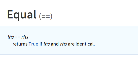
Let's take a look at the documentation page for Equal:

And now, the documentation page for SameQ...

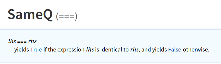
This alone doesn't tell much, but how exactly these two operators (== and ===) are different? The difference lies in their individual strictness.

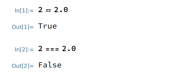
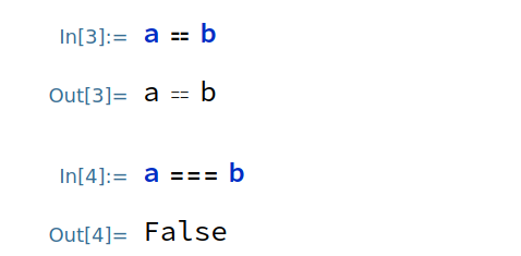
If you want to compare numbers AND their types, use SameQ, if you want less strict comparisons, use Equal.

Sometimes, Equal outputs a symbolic equation, and that can be bad sometimes, if you want to ALWAYS output a boolean value, use SameQ.

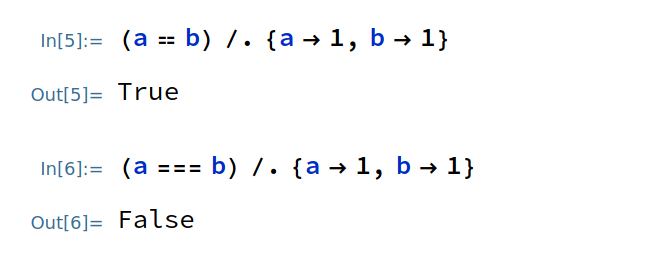
WARNING: SameQ has a higher precedence as an operator. If you want to replace values, replace the values while holding the operation.

If i would get a euro for every time I see horrible/bad approach…

Properties & Relations of constraining a locator

Since the example of constraining a (interactive, or, editable) point or locator to the edge of the unit circle appears over and over again in different yet similar teaching contexts, it can become confusing for the beginner to discern all the coding variations by heart and know which one to use in a given active coding situation. In order to constrain a locator (or point or plot tracker/tracer or alike) key functions can be Locator, LocatorPane, Dynamic, DynamicModule, Manipulate, TrackingFunction, Slider2D, but not all of them at the same time. It depends on what you want and what you start with.

In the end it all boils down to the exploitation of the optional 2nd argument of Dynamic which must be a function (or a list of functions); typically the function is a pure function func[val, expr] processing the "mouse position" (val) and the dynamic expression expr (usually just a single dynamic variable u).

The attached short notebook tries to give a helpful overview of all seven (common) variations for reference and easy comparison.

Also check out the Monday morning quiz testing your beginner's Wolfram L vocabulary!

Attachments:

exampleConstrain...nb

Numerical vs Symbolic -- What to do when plots are blank (and other strange errors)

The plotting functions require numerical inputs. This sounds obvious but most people have trouble debugging plots that come out empty. When something does not plot, the first thing to do is to evaluate the expression and look for undefined variables or typos.

Consider the following:

A = 12;
b = 3;
expr = a* b sin[theta];
Plot[expr, {theta, 0, 10}]

which yields a less than informative plot:

The best approach is to take the plot argument and evaluate it at a point somewhere in the plot range and see that it is numerical. It is often a good idea to evaluate it at the two extremes and the middle to make sure it is numerical everywhere.

expr /. theta -> 0
expr /. theta -> 5
expr /. theta -> 10

to get

 (* 3 a sin[0] 
3 a sin[5] 
3 a sin[10] *)

It becomes clear that the a is undefined and that sin does not evaluate (because of the lower case 's')

Consider Reap/Sow Instead of AppendTo

When using the output of a program to build large lists, a combination of Reap and Sow is often cited as the most efficient (computationally speaking) approach. Put simply, AppendTo trades speed in favour of flexibility by creating a copy of the original list when called. Indeed, Reap/Sow is also point 7 of 10 Tips For Writing Fast Mathematica Code.

I remember first seeing Reap/Sow as a beginner and feeling like it was an 'advanced' feature for other users. Instead I fell into the pattern of defining an empty list and using AppendTo which in hindsight was a beginner's mistake I frequently made by the justification given above.

The example from the link above says it best:

In[7]:= data = {}; 
 Do[AppendTo[data, RandomReal[x]], {x, 0, 40000}]; // AbsoluteTiming

Out[7]= {11.6127, Null}

In[8]:= data = 
   Reap[Do[Sow[RandomReal[x]], {x, 0, 40000}]][[2]]; // AbsoluteTiming

Out[8]= {0.164533, Null}

This is one small change which will Reap large benefits for any beginner.

What does @#(%=<[!} et cetera mean?

Mathematica has a very extensive set of characters used as its syntax. I will try to list most (all?) of them here.

Non-standard characters

If the symbol appears to be a non-standard character one can wrap the symbol in quotes and perform FullForm on it to get the name of the symbol. Example:

gives:

"\[Function]"

Brackets

These syntax elements all appear in pairs:

• (...) Circumfix. Used to group expressions such that it has higher precedence, not used to enclose arguments of a function
• {...} List doc. Circumfix. Used to describe lists of any depth, e.g.: {a,b,...}. Known as arrays, vectors, matrices, tensors, in other languages
• [...] Circumfix. Used to enclose arguments of a function, e.g.: f[a]
• [[...]] Part doc. Post/circumfix. a[[b]] = Part[a,b]. Used to extract parts of an expression. Can also be typeset as a single character: \[LeftDoubleBracket] and \[RightDoubleBracket], and can also be typeset as a subscript
• <|...|> Association doc. Circumfix. Used to describe a list of key-value pairs. Known as associative arrays, dictionaries, hashmaps. Can also be typeset as a single character: \[LeftAssociation] and \[RightAssociation].
• (*...*) Circumfix. Used for making comments in code, can be anywhere in the code except inside strings, then it will be taken literal.
• <*...*> TemplateExpression doc. Circumfix. Expression inside a string template.
• \[LeftFloor]...\[RightFloor] Floor doc. Circumfix. Mathematical Floor function. \[LeftFloor]a\[RightFloor] = Floor[a]. Can be typeset using \[LeftFloor] and \[RightFloor].
• \[LeftCeiling]...\[RightCeiling] Ceiling doc. Circumfix. Mathematical Ceiling function. \[LeftCeiling]a\[RightCeiling] = Ceiling[a]. Can be typeset using \[LeftCeiling] and \[RightCeiling].
• =[...] FreeformEvaluate doc =[query] performs FreeformEvaluate[query]

Applying functions

• @ doc. Infix. Used to apply a function to a single argument: f@x = f[x] (related to Prefix doc)
• // doc. Infix. Used to apply a function to a single argument: x // f = f[x] (related to Postfix doc)
• ~ Infix. Works on two arguments: a ~ f ~ b = f[a,b] (related to Infix doc)
• @* Composition doc. Infix. f@*g = Composition[f,g] Used to compose two or more functions. @* is the infix operator form of Composition
• /* RightComposition doc. Infix. f/*g = RightComposition[f,g] Used to compose two or more functions. /* in the infix operator form of RightComposition
• /@ Map doc. Infix. f/@ a = Map[f,a] Used to apply a function to all elements of a
• //@ MapAll doc. Infix. f//@ a = MapAll[f,a] Used to apply a function to every subexpression of a
• @@ Apply doc. Infix. f @@ a = Apply[f,a] Used to replace the head of a by f
• @@@ Apply doc. Infix. f @@@ a = Apply[f,a,{1}] Used to replace the heads at level 1 of a by f.

Pure function, slots, and slot sequences

• & Function doc. Used to define a pure function where the arguments are given by #1 (short: #), #2, #3, et cetera. Also known as lambda function, anonymous functions, function literal, lambda abstraction...
• # Slot doc. represents the first argument supplied to a pure function
• #1, #2, #n Slot doc. represents the nth argument supplied to a pure function
• #0 Slot doc. represents the pure function itself.
• #name Slot doc. represents the value associated with the key name in an association in the first argument
• ## SlotSequence doc. represents a sequence of all the arguments
• ##n SlotSequence doc. represents a sequence of arguments starting from the nth
• \[Function] Function doc. Infix operator of Function. x \[Function] body = Function[x,body]
• |-> Function doc. Infix operator of Function with names variable. x |-> body = Function[x,body]

Assignments

• = Set doc. Infix. a=b = Set[a,b]
• := SetDelayed doc. Infix. a:=b = SetDelayed[a,b]
• =. Unset doc. Postfix. a=. = Unset[a]
• ^= UpSet doc. Infix. a[b]^=c = Upset[a[b],c]
• ^:= UpsetDelayed doc. Infix. a[b]^:=c = UpSetDelayed[a[b], c]
• /: = TagSet doc. Compound infix. a /: b[a] = c = TagSet[a, b[a], c]
• /: := TagSetDelayed doc. Compound infix. a /: b[a] := c = TagSetDelayed[a, b[a], c]
• /: =. TagUnset doc. Compound infix. a /: b[a] =. = TagUnset[a, b[a]]
• += AddTo doc. Infix. a+=b = AddTo[a, b] Adds b to a and stores the value in a.
• -= SubtractFrom doc. Infix. a-=b = SubtractFrom[a, b] Subtracts b from a and stores the value in a.
• *= TimesBy doc. Infix. a*=b = TimesBy[a, b] Multiplies a by b and stores the value in a.
• /= DivideBy doc. Infix. a/=b = DivideBy[a,b] Divides a by b and stores the value in a.
• //= ApplyTo doc. Infix. a//=f = ApplyTo[a,f]. Applies function f to a and stores the value in a.
• ++ used as a prefix operator is PreIncrement doc. ++a = PreIncrement[a] Adds 1 to a and stores the value in a, returns the new a
• ++ used as a postfix operator is Increment doc. a++ = Increment[a] Adds 1 to a and stores the value in a, returns the old a
• -- used as a prefix operator is PreDecrement doc. --a = PreDecrement[a] Subtracts 1 from a and stores the value in a, returns the new a
• -- used as a postfix operator is Decrement doc. a-- = Decrement[a] Subtracts 1 from a and stores the value in a, returns the old a

Number related

• *^ Infix. Equivalent to *10^ sometimes 'e' in other languages. 3*^4 = 30000
• ` related to Precision doc. Postfix. Define number to be a machine precision number. It denotes context when it is written between symbols. Also appears in pairs inside strings for TemplateSlot doc where they denote an argument
• `n related to Precision doc. Infix. Defines number to have precision n. It denotes context when it is written between symbols
• ``n related to Accuracy doc. Infix. Supposed to be written between 2 numbers. Defines number to have accuracy n
• ^^ related to BaseForm doc. Infix. 3^^1212 represents 1212 written in base 3. Up to base 36 can be specified in this notation (using letters a through z, in either lower of upper case, to denote 10 through 35). Use FromDigits doc for higher bases. Base conversion is done using IntegerDigits doc or RealDigits doc
• \[ImplicitPlus] ImplicitPlus doc. Infix. An invisible character used for e.g. fractions: 5\[ImplicitPlus](3/4) = Plus[5,3/4] = 23/4 where 3/4 is then typed as a fraction

Relational operators

• == Equal doc. Infix. a==b = Equal[a,b]. Used to test if a and b are equal. Also used to define an equation
• \[Equal] Equal doc. Infix. a==b = Equal[a,b]. Used to test if a and b are equal
• != UnEqual doc. Infix a!=b = UnEqual[a,b]. Used to test if a and b are not equal
• ? UnEqual doc. Infix a!=b = UnEqual[a,b]. Used to test if a and b are not equal
• > Greater doc. Infix. a>b = Greater[a,b]. Used to test if a is greater than b
• < Less doc. Infix. a<b = Less[a,b]. Used to test if a is less than b
• >= GreaterEqual doc. Infix. a>=b = GreaterEqual[a,b]. Used to test if a is great than or equal to b
• <= LessEqual doc. Infix. a<=b = LessEqual[a,b]. Used to test if a is less than or equal to b
• === SameQ doc. Infix. a===b = SameQ[a,b]. Used to test if a and b are identical
• =!= UnsameQ doc. Infix. a=!=b = UnsameQ[a,b]. Used to test if a and b are not identical

Note: All the above operator can remain unevaluated, except for SameQ and UnsameQ, these always evaluate to either True or False. Even when a or b is symbolic. All operator can be used multiple times in a row e.g.: a == b == c (all have to be equal) or a > b > c (strictly decreasing numbers) or a != b != c (all unequal). The functions have arbitrary arity, e.g. Equal[] = True.

• \[Element] Element doc. Infix. a \[Element] b = Element[a,b]. Asserts that a is an element of b

Logical operators

• &&, \[And] And doc. Infix. Logical And operator. a && b = a \[And] b = And[a,b] Executes in order and has lazy evaluation
• ||, \[Or] Or doc. Infix. Logical Or operator. a || b = a \[Or] b = Or[a,b] Executes in order and has lazy evaluation
• \[Nand] Nand doc. Infix. Logical Nand operator a \[Nand] b = Nand[a,b] Executes in order and has lazy evaluation
• \[Nor] Nor doc. Infix. Logical Nor operator a \[Nor] b = Nor[a,b] Executes in order and has lazy evaluation
• ! Not doc. Prefix. Logical negation !a = Not[a]. Not to be confused with Factorial doc (postfix operator)
• ¬ Not doc. Prefix. Logical negation ¬a = Not[a].
• \[Xor] Xor doc. Infix. Logical Xor operator a \[Xor] b = Xor[a,b]
• \[Implies] Implies doc. Infix. Logical implication. a \[Implies] b = Implied[a,b]
• \[Equivalent] Equivalent doc. Infix. Logical equivalence testing. a \[Equivalent] b = Equivalent[a,b]

Note: And, Or, Nand, Nor, and Xor have arbitrary arity.

Patterns and rules

• _ Blank doc. Prefix. _ = Blank[]
• _a Blank doc. Prefix. _a = Blank[a]
• __ BlankSequence doc. Prefix. __ = BlankSequence[]
• __a BlankSequence doc. Prefix. __a = BlankSequence[a]
• ___ BlankNullSequence doc. Prefix. ___ = BlankNullSequence[]
• ___a BlankNullSequence doc. Prefix. ___a = BlankNullSequence[a]
• a_ Pattern doc. Postfix/infix. a_ = Pattern[a, Blank[]]
• a:_ Pattern doc. Postfix/infix. a:_ = Pattern[a, Blank[]]
• a__ Pattern doc. Postfix/infix. a__ = Pattern[a, BlankSequence[]]
• a:__ Pattern doc. Postfix/infix. a:__ = Pattern[a, BlankSequence[]]
• a___ Pattern doc. Postfix/infix. a__ = Pattern[a, BlankNullSequence[]]
• a:___ Pattern doc. Postfix/infix. a:__ = Pattern[a, BlankNullSequence[]]
• _. Optional doc. Postfix. _. = Optional[Blank[]] also related to Default doc
• _:a Optional doc. Postfix. _:a = Optional[Blank[],a] also related to Default doc
• __. Optional doc. Postfix. __. = Optional[BlankSequence[]] also related to Default doc
• __:a Optional doc. Postfix. __:a = Optional[BlankSequence[],a] also related to Default doc
• ___. Optional doc. Postfix. ___. = Optional[BlankNullSequence[]] also related to Default doc
• ___:a Optional doc. Postfix. ___:a = Optional[BlankNullSequence[],a] also related to Default doc
• /; Condition doc. Infix. a /; b = Condition[a, b]
• ? PatternTest doc. Infix. a ? b = PatternTest[a,b]
• -> Rule doc. Infix. a -> b = Rule[a,b]
• \[Rule] Rule doc. Infix. a \[Rule] b = Rule[a,b]
• :> RuleDelayed doc. Infix. a :> b = RuleDelayed[a,b]
• \[RuleDelayed] RuleDelayed doc. Infix. a \[RuleDelayed] b = RuleDelayed[a,b]
• /. ReplaceAll doc. Infix. a /. b = ReplaceAll[a, b]
• //. ReplaceRepeated doc. Infix. a //. b = ReplaceRepeated[a,b]
• .. Repeated doc. Postfix. a.. = Repeated[a]
• ... RepeatedNull doc. Postfix. a... = RepeatedNull[a]
• | Alternatives doc. Infix. a | b = Alternatives[a, b]. Not to be confused with || Or doc

String related

• <> StringJoin doc. Infix. a<>b = StringJoin[a,b]
• ~~ StringExpression doc. Infix. a~~b = StringExpression[a,b]

Note: both have arbitrary arity.

Graph related

• <-> UndirectedEdge doc. Infix. a<->b = UndirectedEdge[a,b]
• \[UndirectedEdge] UndirectedEdge doc. Infix. a\[UndirectedEdge]b = UndirectedEdge[a,b]
• \[DirectedEdge] DirectedEdge doc. Infix. a\[DirectedEdge]b = DirectedEdge[a,b]

Other

• \[Application] Application doc a\[Application]b Performs Application[a,b].
• . Dot doc a.b Performs the dot product of a and b
• , Used to separate arguments in a function call, e.g.: f[a,b]
• % Out doc. % = Out[$Line - 1] = Out[]. Gives the last result generated
• %% Out doc. %% = Out[-2]. Gives the penultimate result
• %..% (k repetitions of %) Out doc. %...% = Out[-k]. Gives the k-th last result
• %n Out doc. Gives the result of line n
• \[PartialD] D doc. Postfix. Use in combination with a subscript to denote a partial derivate
• \[DifferentialD] Integrate doc. Compound match fix. \[Integral]a\[DifferentialD]b = Integrate[f,b]
• ! as a postfix operator means Factorial doc a! = Factorial[a]. Mathematical factorial function
• !! as a postfix operator means Factorial2 doc a!! = Factorial2[a]. Mathematical double factorial function
• ; CompoundExpression doc. Infix. a=1;a=2 = CompoundExpression[a=1,b=2] Though it might look like a postfix operator, it is not: a=1;a=2; = CompoundExpression[a=1,b=2,Null]
• ;; Span doc. Infix. a ;; b = Span[a,b] and a ;; b ;; c= Span[a,b,c] Note that more than 2 infix operator in a row will give (most likely) unexpected results
• :: MessageName doc. Infix. a::b = MessageName[a,b]
• ? Information doc. Prefix. ?a = Information[f, LongForm -> False]. Print some information about symbol a
• ?? Information doc. Prefix. ??a = Information[f]. Print information about symbol a
• << Get doc. Prefix. << a = Get["a"]. Reads in file a, evaluating each expression in it and returning the last one. Not to be confused with left bit shift operators in other languages (BitShiftLeft doc)
• >> Putt doc. Infix. a >> b = Put[a,b]. Write a to file b. Not to be confused with right bit shift operators in other languages (BitShiftRight doc)
• >>> PutAppend doc. Infix. a >>> b = PutAppend[a,b]. Appends a to file b.

In case some symbol(s) is(are) missing, let me know!

Thanks, had added a previous version of ApplyTo, now fixed, and also added [Application]. (https://reference.wolfram.com/language/ref/Application.html)

Also added this explicitly. thanks!

Not sure how you are entering the left and right floor brackets but that is the problem,

\[LeftFloor]5.5\[RightFloor]
(* 5 *)

To enter from the keyboard esclfesc and escrfesc where esc is escape.

Basic syntax of built-in functions

• All built-in functions start from capital letters and are in CamelCase for compound names. Users of many other programming languages might miss this as they are used to different conventions. Examples: Plot, ListPlot, FindSpanningTree, etc.

• Arguments of a function are inclosed in square brackets. Round parenthesis are used only for ordering of operations. Again, other languages use different conventions. Examples:

  • Cos[Pi] --- is a function with a single argument Pi.
  • BesselJ[1/2, 5] --- is a function with 2 arguments
  • (2-Cos[Pi])Sin[Pi/3] --- round parenthesis are used to order operations