General information and download links
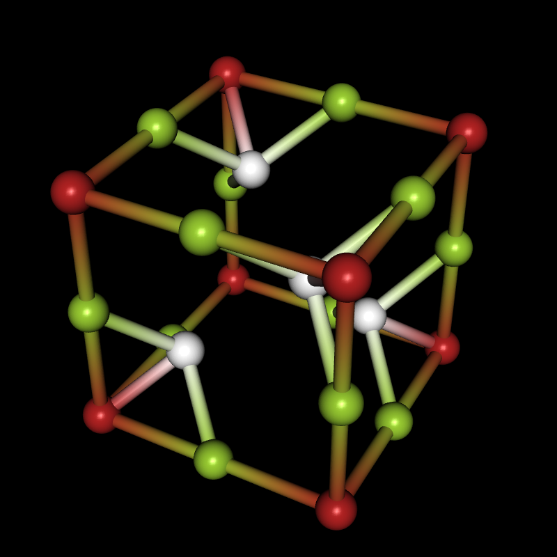
If you're interested in crystal structures, you can now download the Crystallica application from the Wolfram Library Archive, and then you can do things like this:
Needs["Crystallica`"];
CrystalPlot[
{{5.4,0,0},{0,5.4,0},{0,0,5.4}},
{{0,0,0},{0,0,.5},{0,.5,0},{.5,0,0},{.24,.24,.24},{.24,.76,.76},{.76,.24,.76},{.76,.76,.24}},
{1,2,2,2,3,3,3,3},
AtomCol->{"Firebrick","YellowGreen",White},AtomRad->.4,
BondStyle->2,BondDist->3,
CellLineStyle->False,AddQ->True,Lighting->{{"Directional",White,ImageScaled[{0,0,1}]}},Background->Black]
Here are the download links for Crystallica and two other packages you may need:
Crystallica - contains the functions CrystalPlot and CrystalChange
CifImport - contains an import function for CIF files
VaspImport - contains an import function for files related to VASP
Once you've installed Crystallica (by saving the entire Crystallica folder - not the zip archive - to $USerBaseDirectory/Applications and re-starting the Kernel), you can enter Crystallica into the Documentation Center and you'll find lots of useful examples. Most of the examples in this post are taken from the Documentation. For the other two packages, just install them and evaluate this:
?CifImport
?VaspImport
I'll first show you a few things the CrystalPlot function can do when you already have crystal structure data inside Mathematica, wherever it may have come from. Then we'll take a look at how to get the data into Mathematica in the first place, which is where CifImport and VaspImport will come into play - but we'll get data from other sources as well. I'll cover the different import solutions in separate replies to this thread, because I have a feeling that I'll be rambling on and on and on...
Simple plot
Traditional ball-and-stick plots are usually just fine, so the simplest thing you can do is this:
CrystalPlot[
{{4.5,0,0},{0,4.5,0},{0,0,3}},
{{0,0,0},{.5,.5,.5},{.2,.8,.5},{.3,.3,0},{.7,.7,0},{.8,.2,.5}},
{1,1,2,2,2,2}]
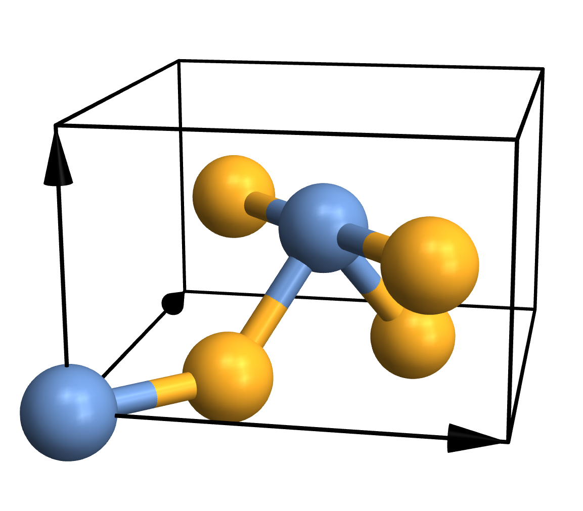
As you can see, CrystalPlot expects three arguments. The first one contains the lattice vectors, which are simply the three vectors that create the parallelepiped that constitutes the cell. The second argument contains the atomic coordinates, but they're given in the basis of the lattice vectors (which is quite useful in crystallography). The third argument is a list of integers that gives the atom types, with one entry for each atom. If you want to plot a molecule instead, you can call CrystalPlot with just two arguments: A list of atom coordinates in cartesian space, and a list of atom types. Everything else you see in the plot - the atoms, bonds, colours, arrows etc. - represents the default settings of various layout options.
Advanced atoms and bonds
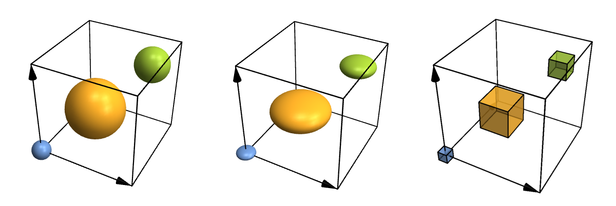
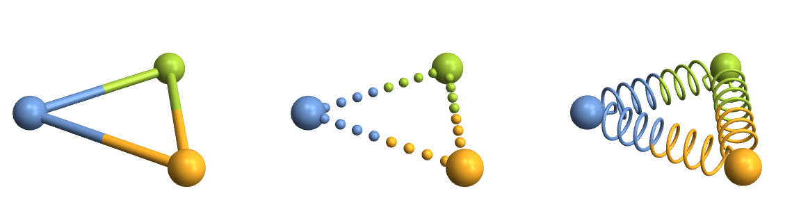
Let's take a look at some more advanced options just for fun. For instance, atoms and bonds can look any way you need them to, because you can specify your own functions for them. You can also fine-tune where to put bonds and what to do with their thickness and colour in a physically (or chemically) meaningful way, but I won't show that here. So here are some customized atoms and bonds:
Row[Table[
CrystalPlot[{{4,0,0},{0,4,0},{0,0,4}},{{0,0,0},{.4,.4,.4},{.8,.8,.8}},{1,2,3},
AtomRad->{.4,1.2,.7},AtomFunction->style,ImageSize->400],
{style,{
(Ball[#1,#2]&),
(Scale[Sphere[#1,#2],{1,1,.5}]&),
({EdgeForm[Thick],Opacity[.7],Cuboid[#1-.5*#2,#1+.5*#2]}&)
}}]]
Row[Table[
CrystalPlot[{{0,0,0},{5,0,0},{2.5,4,0}},{1,2,3},BondDist->6,BondStyle->style,ImageSize->400],
{style,{
1,
Function[{bonds,partcol},Table[{If[ii<.5,partcol[#,1],partcol[#,2]],Sphere[bonds[[#,1]]+ii*(bonds[[#,2]]-bonds[[#,1]]),.15]},{ii,0,1,1/9}]&/@Range[Length[bonds]]],
Function[{bonds,partcol},Module[{spiral,points,rad=.05},
spiral[atoms_]:=Module[{scale=.5,dist=atoms[[2]]-atoms[[1]],curls=60,normal,rot,scaled},
normal=Table[{scale*Cos[ii],scale*Sin[ii],.1*ii},{ii,0,curls,\[Pi]/10}];
scaled={#[[1]],#[[2]],10*Norm[dist]/curls*#[[3]]}&/@normal;
rot=scaled.Quiet[RotationMatrix[{dist,{0,0,1}}]];
Join[{atoms[[1]]},#+atoms[[1]]&/@(rot[[25;;-25]]),{atoms[[2]]}]];
points=spiral/@bonds;
{partcol[#,1],Tube[BSplineCurve[points[[#,;;Round[Length[points[[#]]]/2]]],rad]],partcol[#,2],Tube[BSplineCurve[points[[#,Round[Length[points[[#]]]/2];;]],rad]]}&/@Range[Length[bonds]]
]]
}}]]
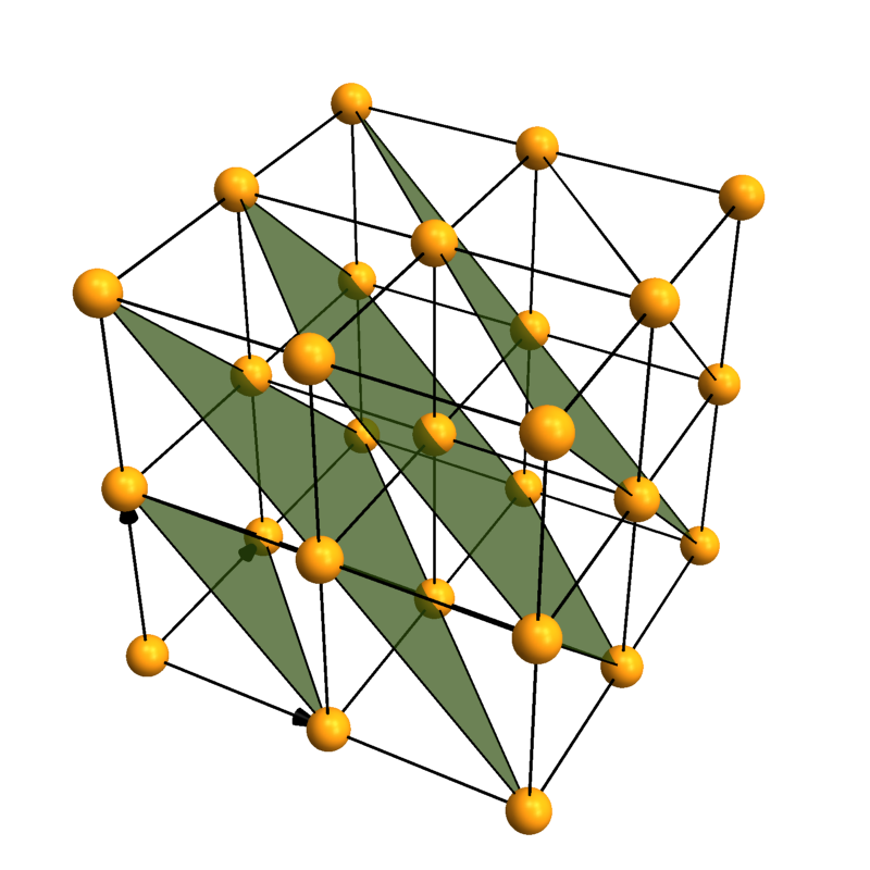
Lattice planes
Crystallica can also add lattice planes to the plot. You can specify them using [h,k,l] Miller indices and distance to the origin.
CrystalPlot[{{3,0,0},{0,3,0},{0,0,3}},{{0,0,0}},{1},
AddQ->True,AtomRad->.3,AtomCol->"CadmiumYellow",Sysdim->2,CellLineStyle->2,
LatticePlanes->Table[{{1,1,1},dist},{dist,1,5}],ContourStyle->{"TerreVerte",Opacity[.7]},BoundaryStyle->Thick]
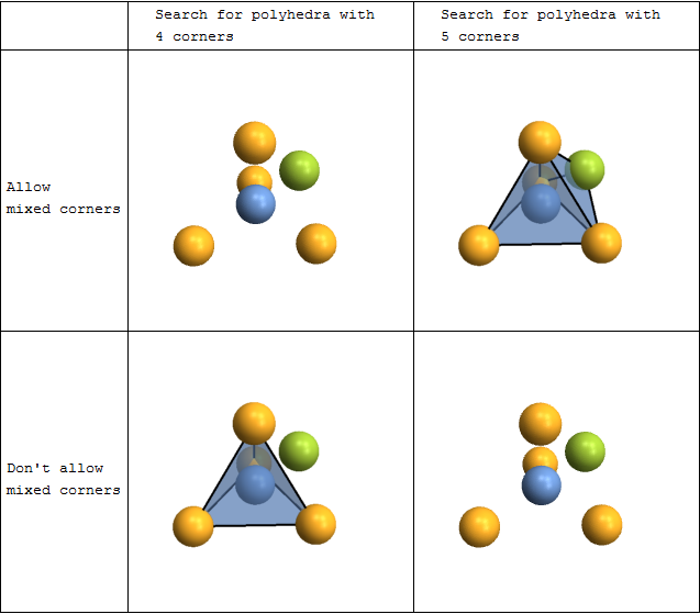
Coordination polyhedra
You can automatically search for and plot coordination polyhedra. This is not limited to the commonly occurring tetrahedra and octahedra - you can actually look for polyhedra with arbitrary numbers of corners. There are also options to fine-tune both the searching and the rendering.
plot[corners_,mixed_]:=CrystalPlot[{{0,0,0},{0,0,1.8},{-.9,-1.5,-.6},{-.9,1.5,-.6},{1.7,0,-.6},{.8,.8,.8}},{1,2,2,2,2,3},
BondStyle->False,ImageSize->250,
PolyMode[corners]->{"Show"->All,"AllowMixed"->mixed},PolyStyle[corners]->Directive[Opacity[.5],EdgeForm[Thick]]];
Grid[{{
"",
"Search for polyhedra with \n4 corners",
"Search for polyhedra with \n5 corners"
},{
"Allow \nmixed corners",
plot[4,True],
plot[5,True]
},{
"Don't allow \nmixed corners",
plot[4,False],
plot[5,False]
}},Dividers->All]
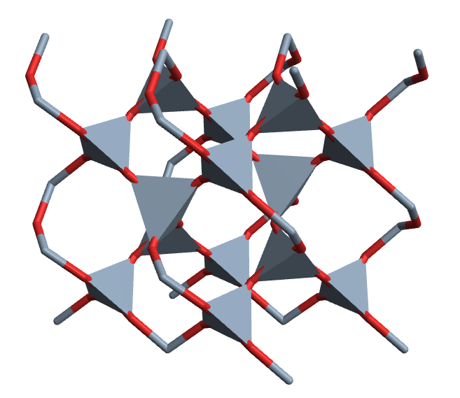
CrystalPlot[{{2.5,-4.3,0},{2.5,4.3,0},{0,0,5.5}},
{{.5,0,0},{0,.5,.7},{.5,.5,.3},{.2,.4,.5},{.6,.8,.2},{.2,.8,.8},{.8,.6,.5},{.4,.2,.2},{.8,.2,.8}},{1,1,1,2,2,2,2,2,2},
PolyMode[4]->True,PolyStyle[4]->EdgeForm[None],AddQ->True,
Sysdim->2,AtomRad->0,CellLineStyle->False,AtomCol->{"SlateGray","Firebrick"},
ViewAngle->.4,ViewPoint->{3.2,0,1.1},ViewVertical->{.5,0,1.2}]
Other things
Visualization aside, you can also build supercells, change cell shapes, or add, remove and sort atoms... but that's a bit boring to read, so I'll refer you to the Documentation page of the CrystalChange function instead.
If you're interested, we can use this thread to talk about any questions you may have, or you can share your use of the package (if you decide to use it). I'm not offering full support here, but I'll be floating around, and I'd like to hear your feedback. We don't have any intentions to be involved in further development. But if you have a good idea and some time, then by all means, work on it for yourself, or host it on your favourite code collaboration site.
Bianca Eifert and Christian Heiliger


