Message Boards Message Boards

Walking strandbeest dynamics

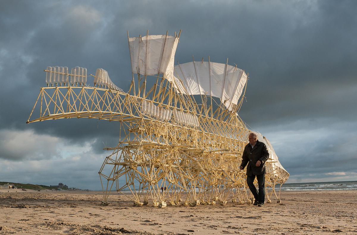
Many of you have seen the strandbeest (from Dutch, meaning beach-beast). These PVC tube animals created by Theo Jansen walk along the beach and are wind powered:

enter image description here

Years ago (2009 to be more exact) I made a post on my blog about the movement of the legs, as evidenced by the still-nicely-working Mathematica notebook:

enter image description here

At the time the proportions of the legs were not known publicly so I meticulously studied frames of (low quality) YouTube videos. I made the following diagram in Illustrator of what I thought I saw:

enter image description here enter image description here

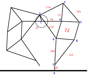
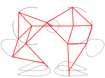
On the left the length of the legs in red, and in blue the numbers of the joints. On the right the trajectory of the joints that I calculated at the time in Mathematica. It's funny that my blog does not exist any more (for years actually), but these images live on, as I found out when I looked for strandbeest on Google Images:

enter image description here

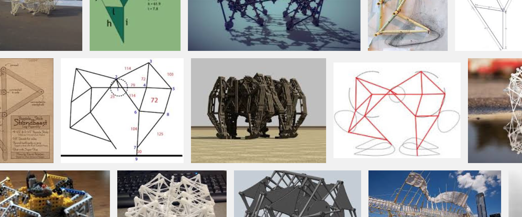
My images! But not on my website! Nice to see people still use it. Now, in 2016, I saw these files on my laptop, and thought: is there finally more known about them? Well yes, there is! The exact proportions are now known and there is tons and tons of videos, lectures, 3D-printable strandbeest models, interviews with Theo Jansen and other stuff! So now we can find the exact dimensions readily on the internet:

enter image description here

Notice that I (wrongly) assumed that the legs had 'feet'! oops! I was very happy to see that my lengths were not that wrong though! Let's recreate the strandbeest. We do so by first creating a function that quickly finds the intersection of two circles:

Clear[FindPoint, FindLines]
FindPoint[p1 : {x1_, y1_}, p2 : {x2_, y2_}, R_, r_, side_] := Module[{d, x, y, vc1, vc2, p, sol, sol1, sol2, s1, s2, sr},
  d = N@Sqrt[(x2 - x1)^2 + (y2 - y1)^2];
  x = (d^2 - r^2 + R^2)/(2 d);
  y = Sqrt[R^2 - x^2];
  vc1 = Normalize[{x2 - x1, y2 - y1}];
  vc2 = Cross[vc1];
  p = {x1, y1} + x vc1;
  {sol1, sol2} = {p + y vc2, p - y vc2};
  s1 = Sign[Last[Cross[Append[(p2 - p1), 0], Append[(sol1 - p1), 0]]]];
  s2 = Sign[Last[Cross[Append[(p2 - p1), 0], Append[(sol2 - p1), 0]]]];
  sr = If[side === Left, 1, -1];
  Switch[sr, s1,
   sol1
   ,
   s2
   ,
   sol2
   ]
  ]

This finds on the side 'side' (Left/Right) the intersection point of two circles positioned at p1 and p2, with radii R and r, respectively. And now we can easily compute all the little vertices/joints of our beast:

FindLines[\[Theta]_] := Module[{p1, p2, p3, p4, p5, p6, p7, p8, p10, p11, p12, p13, p14, p15},
  {p1, p2, p3, p4, p5, p6, p7, p8, p10, p11, p12, p13, p14, p15} = FindPoints[\[Theta]];
  {{p1, p2}, {p2, p3}, {p3, p4}, {p1, p4}, {p2, p6}, {p4, p6}, {p3, p5}, {p4, p5}, {p5, p8}, {p6, p8}, {p6, p7}, {p7, p8}, {p1, 
    p11}, {p10, p11}, {p2, p10}, {p2, p13}, {p11, p13}, {p10, p12}, {p11, p12}, {p12, p14}, {p13, p14}, {p13, p15}, {p14, p15}}
  ]
FindPoints[\[Theta]_] := Module[{p1, p2, p3, p4, p5, p6, p7, p8, p9, p10, p11, p12, p13, p14, p15, p16},
  p1 = {0, 0};
  p4 = {38, -7.8};
  p11 = {-38, -7.8};
  p2 = 15 {Cos[\[Theta]], Sin[\[Theta]]};

  p3 = FindPoint[p2, p4, 50, 41.5, Left];
  p6 = FindPoint[p2, p4, 61.9, 39.3, Right];
  p5 = FindPoint[p3, p4, 55.8, 41.5, Left];
  p8 = FindPoint[p5, p6, 39.4, 36.7, Left];
  p7 = FindPoint[p6, p8, 49, 65.7, Right];

  p10 = FindPoint[p2, p11, 50, 41.5, Right];
  p13 = FindPoint[p2, p11, 61.9, 39.3, Left];
  p12 = FindPoint[p10, p11, 55.8, 41.5, Right];
  p14 = FindPoint[p12, p13, 39.4, 36.7, Right];
  p15 = FindPoint[p13, p14, 49, 65.7, Left];

  {p1, p2, p3, p4, p5, p6, p7, p8, p10, p11, p12, p13, p14, p15}
  ]

Now we can plot it easily:

trajectoriesdata = (FindPoints /@ Subdivide[0, 2 Pi, 100])\[Transpose];
Manipulate[
  Graphics[{Arrowheads[Large], Arrow /@ trajectoriesdata, Thick, Red, Line[FindLines[\[Theta]]]},
   PlotRange -> {{-150, 150}, {-120, 70}}, 
   ImageSize -> 800
  ]
 ,
 {\[Theta], 0, 2 \[Pi]}
]

enter image description here

We can also make an entire bunch of legs at the same time and make a 3D beast!

Manipulate[
 mp = 60;
 n = 12;
 \[CurlyPhi] = Table[Mod[5 \[Iota], n, 1], {\[Iota], 1, n}];
 Graphics3D[{Darker@Yellow, Table[
    Line[ 
     Map[Prepend[mp \[Iota]], 
      FindLines[\[Theta] + \[CurlyPhi][[\[Iota]]] (2 Pi/n)], {2}]],
    {\[Iota], n}
    ]
   , Black, Line[{{mp 1, 0, 0}, {mp n, 0, 0}}]
   }
  ,
  Lighting -> "Neutral",
  PlotRangePadding -> Scaled[.1],
  PlotRange -> {{-mp, (n + 1) mp}, {-150, 150}, {-150, 150}},
  Boxed -> False,
  ImageSize -> 700
  ]
 ,
 {\[Theta], 0, 2 \[Pi]}
 ]

enter image description here

From the side we can look at how the legs of 4-pair-legged and 6-pair-legged versions of the beasts work:

enter image description here enter image description here

Hope you enjoyed this! Perhaps someone else can make this thing actually walk over a (bumpy) surface?

POSTED BY: Sander Huisman
14 Replies

This work may be known to those in this thread, but a research group at Disney developed a nice program to compute the gearing mechanisms required to approximate a motion curve specified by the user:

Stelian Coros, Bernhard Thomaszewski, Gioacchino Noris, Shinjiro Sueda, Moira Forberg, Robert W. Sumner, Wojciech Matusik, and Bernd Bickel. 2013. Computational design of mechanical characters. ACM Trans. Graph. 32, 4, Article 83 (July 2013), 12 pages.

I seem to recall they released a computer program as well, but now I can't find it. The same lab (but mostly different researchers) designed a similar system for kinetic wire characters:

Hongyi Xu, Espen Knoop, Stelian Coros, and Moritz Bächer. 2018. Bend-it: design and fabrication of kinetic wire characters. ACM Trans. Graph. 37, 6, Article 239 (December 2018), 15 pages.

POSTED BY: Robert Jacobson

An interesting variation with genetic algorithms used to improve the linkage. I could not find more detailed info though. I think it was 3D printed and is highly maneuvering.

The City Beest by Hans Jørgen Grimstad

enter image description here

POSTED BY: Vitaliy Kaurov

Theo Jansen, the strandbeest inventor, actually also used evolutionary algorithms on an Atari (!!) that made 1500 perturbation of a known state, then keep 150, make for each of them 10 perturbations and keep 150, and do this several times. It took many months on this Atari to run!

POSTED BY: Sander Huisman
Posted 8 years ago

Here are the links to some demonstrations about walking machine mechanisms I made some time ago:

Chebyshev Walking Machine

Walking Mechanism Using a Klann Linkage

These are in fact all variations of coupler curves of the 4-bar linkage and like mechanisms. Here is a link to my demonstration about this:

Coupler Curves of a Four-Bar Linkage

In fact, almost any curve can be generated by some mechanical linkage. See more of these demonstrations: Polar Curve Generator with Five-Bar Linkage

Designs from Mechanical Linkages

Back in 1951, Hrones and Nelson made an comprehensive atlas of about 10,000 coupler curves that can be obtained by changing the parameters. This was (and is) used to construct a mechanism adapted to generate a desired curve with a specific position and speed variation along it.

I am preparing another demonstration that can generate all curves as explored in the Hrones and Nelson atlas. This gives an idea of the curves/ speed combinations that can be generated. The walking machine mechanisms are part of these. Just find a parameter (bar dimension) combination with a sufficient straight line/constant speed section.

Coupler curve atlas generator

Coupler Curve Atlas: Analysis of the four-bar linkage

POSTED BY: Erik Mahieu

In the spirit of the original T. Jensen art I think it is a good idea to use XKCD styling of the graphics:

enter image description here

Here is the code (using modifications of Mr.Wizard's answer at MSE):

(*********************************)
(* Mr.Wizard's code for XKCD style*)
(*********************************)

split[{a_, b_}] := 
 If[a == b, {b}, 
  With[{n = Ceiling[3 Norm[a - b]]}, Array[{n - #, #}/n &, n].{a, b}]]

partition[{x_, y__}] := Partition[{x, x, y}, 2, 1]

nudge[L : {a_, b_}, d_] := Mean@L + d Cross[a - b];

gap = {style__, x_BSplineCurve} :> {{White, AbsoluteThickness[10], x}, style, 
    AbsoluteThickness[2], x};

wiggle[pts : {{_, _} ..}, 
  d_: {-0.15, 0.15}] := ## &[#~nudge~RandomReal@d, #[[2]]] & /@ 
  partition[Join @@ split /@ partition@pts]

xkcdify[plot_Graphics] := 
 Show[FullGraphics@plot, TextStyle -> {17, FontFamily -> "Humor Sans"}] /. 
   Line[pts_] :> {AbsoluteThickness[2], BSplineCurve@wiggle@pts} // 
  MapAt[# /. gap &, #, {1, 1}] &

(* Modification *)
xkcdify[plot : (Line | Arrow)[_], d_: {-0.15, 0.15}] :=
  Block[{funcHead = Head[plot], bf = BSplineCurve},
   If[funcHead === Arrow, bf = Arrow@*bf];
   plot /. funcHead[pts_] :> {AbsoluteThickness[2], bf@(wiggle[#, d] &)@pts} //
     MapAt[# /. gap &, #, {1, 1}] &
   ];

(******************************)
(* Sander's code modification *)
(******************************)

rescaleRule = {x_?NumericQ, y_?NumericQ} :> {Rescale[x, {-150, 150}, {-3, 3}],
    Rescale[y, {-120, 50}, {-2.5, 1}]}; FindLines[0.4] /. rescaleRule;

trajectoriesdata = (FindPoints /@ Subdivide[0, 2 Pi, 100])\[Transpose];
trajectoriesdataXKCD = 
  Map[xkcdify[Arrow[#], {-0.23, 0.23}] &, (trajectoriesdata /. 
     rescaleRule)];
man = Manipulate[
  Graphics[{Arrowheads[Large], trajectoriesdataXKCD, Thick, Red, 
    Map[xkcdify[Line[#], {-0.1, 0.1}] &, 
     FindLines[\[Theta]] /. rescaleRule]}, Frame -> True, 
   PlotRange -> {{-3, 3}, {-3, 1}}, ImageSize -> 800], {\[Theta], 0, 
   2 \[Pi]}, AutorunSequencing -> {Automatic, 5}]
POSTED BY: Anton Antonov

Haha nice combination! thanks for sharing!

POSTED BY: Sander Huisman

Hi Sander,

thank you very much for sharing this nice code - I already had a lot of fun playing around with it! I have just a little remark to make: It seems to me that in your function FindPoints there is a typo; it should read (see comments, c.f. line "d"):

FindPoints[\[Theta]_] := 
 Module[{p1, p2, p3, p4, p5, p6, p7, p8, p9, p10, p11, p12, p13, p14, 
   p15, p16},
  p1 = {0, 0};
  p4 = {38, -7.8};
  p11 = {-38, -7.8};
  p2 = 15 {Cos[\[Theta]], Sin[\[Theta]]};
  p3 = FindPoint[p2, p4, 50, 41.5, Left];
  p6 = FindPoint[p2, p4, 61.9, 39.3, Right];
  p5 = FindPoint[p3, p4, 55.8, 40.1(*41.5*), Left];
  p8 = FindPoint[p5, p6, 39.4, 36.7, Left];
  p7 = FindPoint[p6, p8, 49, 65.7, Right];
  p10 = FindPoint[p2, p11, 50, 41.5, Right];
  p13 = FindPoint[p2, p11, 61.9, 39.3, Left];
  p12 = FindPoint[p10, p11, 55.8, 40.1(*41.5*), Right];
  p14 = FindPoint[p12, p13, 39.4, 36.7, Right];
  p15 = FindPoint[p13, p14, 49, 65.7, Left];
  {p1, p2, p3, p4, p5, p6, p7, p8, p10, p11, p12, p13, p14, p15}]

Then the resulting trajectory of the foot motion (along the ground) looks better:

enter image description here

Best regards -- Henrik

POSTED BY: Henrik Schachner

oops! one length is wrong! Well, easy to correct ;) Thanks for spotting!

POSTED BY: Sander Huisman

Here a bit nicer with small figures:

enter image description here

And as an animation:

enter image description here

Notebook as attachment. (can now be ran by just executing the entire notebook).

Attachments:
POSTED BY: Sander Huisman

enter image description here - another post of yours has been selected for the Staff Picks group, congratulations !

We are happy to see you at the tops of the "Featured Contributor" board. Thank you for your wonderful contributions, and please keep them coming!

POSTED BY: Moderation Team

For 6 pairs of legs (seen in many build-kits), with the phase difference of each successive pairs of legs just being Pi/3, you will get the following animation:

enter image description here

where I marked each pair by number and by F(front) and B(back).

The trajectory of one of the feet can be obtained like so:

pts = Subdivide[0, 2 Pi, 150];
trajectoriesdata = (FindPoints /@ pts)\[Transpose];
trajectoriesdata = trajectoriesdata[[-1]];
Graphics[{Arrow[trajectoriesdata], Point[trajectoriesdata]}, Axes -> True]

enter image description here

To get the angles when it touching we find the minima and maxima in X position:

ClearAll[XPosFeet,XPosFeet2]
XPosFeet[\[Theta]_?NumericQ]:=FindPoints[\[Theta]][[-1,1]]
XPosFeet2[\[Theta]_?NumericQ]:=FindPoints[\[Theta]][[7,1]]
min\[Theta]=\[Theta]/.Quiet@FindMaximum[XPosFeet[\[Theta]],{\[Theta],2,1,3}][[2]];
max\[Theta]=\[Theta]/.Quiet@FindMinimum[XPosFeet[\[Theta]],{\[Theta],4.5,3,6}][[2]];
{min\[Theta]2,max\[Theta]2}={\[Pi]/2+(\[Pi]/2-min\[Theta]),3\[Pi]/2+(3\[Pi]/2-max\[Theta])}

ClearAll[LeftOnGroundQ,RightOnGroundQ]
LeftOnGroundQ[\[Theta]_?NumericQ]:=!(min\[Theta]<Mod[\[Theta],2\[Pi]]<max\[Theta])
RightOnGroundQ[\[Theta]_?NumericQ]:=min\[Theta]2<Mod[\[Theta],2\[Pi]]<max\[Theta]2

Plot[XPosFeet[\[Theta]],{\[Theta],0,2\[Pi]},GridLines->{{min\[Theta],max\[Theta]},{}}]
Plot[XPosFeet2[\[Theta]],{\[Theta],0,2\[Pi]},GridLines->{{\[Pi]/2+(\[Pi]/2-min\[Theta]),3\[Pi]/2+(3\[Pi]/2-max\[Theta])},{}}]
Manipulate[Graphics[{Red,Line[FindLines[\[Theta]]],If[LeftOnGroundQ[\[Theta]],Disk[{-50,-100}],{}],If[RightOnGroundQ[\[Theta]],Disk[{50,-100}],{}]},PlotRange->{{-150,150},{-120,70}},ImageSize->800],{\[Theta],0,2\[Pi]}]

giving:

enter image description here

where the dot now indicates touching.

Now we can do some bigger code to generate a nice diagram:

mp=60;
n=6;
(*\[CurlyPhi]=Table[Mod[5\[Iota],n,1],{\[Iota],1,n}];*)
\[CurlyPhi]=Range[n];
Manipulate[
    Graphics3D[{Darker@Yellow,Table[
        {
        Line[ Map[Prepend[mp \[Iota]],FindLines[\[Theta]+\[CurlyPhi][[\[Iota]]] (2Pi/n)],{2}]],
        {Black,Text[\[Iota],{mp \[Iota],0,50}]}
        },
        {\[Iota],n}
    ]
    ,Black,Line[{{mp 1,0,0},{mp n,0,0}}]
    ,MapThread[Text[#1,{mp (n+1),#2,-100}]&,{{"F","B"},{-50,50}}]
    }
    ,
    Lighting->"Neutral",
    PlotRangePadding->Scaled[.1],
    PlotRange->{{-mp,(n+1)mp},{-150,150},{-150,150}},
    Boxed->False,
    ImageSize->700
    ]
,
{\[Theta],0,2\[Pi]}
]

separators={min\[Theta],max\[Theta],min\[Theta]2,max\[Theta]2};
separators=Table[separators-\[CurlyPhi][[\[Iota]]],{\[Iota],n}];
separators=Mod[Flatten[separators],2\[Pi]];
separators=separators//Prepend[0.0]//Append[2.0\[Pi]];
separators=Union[separators];
regions=Partition[separators,2,1];
expanded=Partition[Subdivide[0,2\[Pi],regions//Length],2,1];

ClearAll[MakeRegionPart]
MakeRegionPart[{\[Theta]start_,\[Theta]stop_},{start_,stop_}]:=Module[{eval,onground,ypos,xpos,pos,support},
    eval=(\[Theta]start+\[Theta]stop)/2.0;
    onground=Table[{LeftOnGroundQ[eval+\[CurlyPhi][[\[Iota]]]],RightOnGroundQ[eval+\[CurlyPhi][[\[Iota]]]]},{\[Iota],n}];
    xpos=Subdivide[start,stop,3][[2;;-2]];
    ypos=Subdivide[0.5,0,n+1][[2;;-2]];
    pos=Partition[Reverse/@Tuples[{ypos,xpos}],2];
    support=MapThread[If[#1,Disk[#2,0.02],{}]&,{onground,pos},2];
    (*Print[support];*)
    {
        Line[{{{\[Theta]start,0.75},{\[Theta]start,1.25}},{{\[Theta]stop,0.75},{\[Theta]stop,1.25}}}],
        Line[{{{start,0},{start,0.5}},{{stop,0},{stop,0.5}}}],
        {Dashed,Opacity[0.5],Line[{{{\[Theta]start,0.75},{start,0.5}},{{\[Theta]stop,0.75},{stop,0.5}}}]},
        support
    }
]

xpos1=Subdivide[Sequence@@expanded[[1]],3][[2;;-2]];
ypos1=Subdivide[0.5,0,n+1][[2;;-2]];

Graphics[{
    MapThread[MakeRegionPart,{regions,expanded}],
    Text[#,{#,1.35}]&/@Range[0,2\[Pi],\[Pi]/2],
    MapThread[Text[#1,{#2,-0.1}]&,{{"F","B"},xpos1}],
    MapThread[Text[#1,{-0.1,#2}]&,{Range[n],ypos1}]
}
]
(*
plts=Table[
Plot[{If[LeftOnGroundQ[\[Theta]+\[CurlyPhi][[\[Iota]]]],20-4\[Iota],Missing[]],If[RightOnGroundQ[\[Theta]+\[CurlyPhi][[\[Iota]]]],20-(4\[Iota]+1),Missing[]]},{\[Theta],0,2\[Pi]}]
,
{\[Iota],n}
];
Show[plts,PlotRange\[Rule]All,GridLines\[Rule]{separators,{}},AspectRatio->1/5,ImageSize\[Rule]1000]*)

Giving:

enter image description here

I attached my notebook so you can change the number of feet and the relative phases between the legs... Note that this notebook was not meant to be easily understood ;-)

Attachments:
POSTED BY: Sander Huisman

@Sander Huisman amazing post! I also would like to point to two demonstrations on the subject, see below. @Marco Thiel, indeed an interesting exciting idea about gait pattern. Sander, do you think we really have to adapt to 12, - is due to instability or inefficiency of this strandbeest with 4 legs? Perhaps it could walk with 4?

Jansen Walker by Contributed by Karl Scherer, Additional contributions: Theo Jansen

A Theo Jansen Walking Linkage by Sándor Kabai

enter image description here

enter image description here

POSTED BY: Vitaliy Kaurov

Hi Sander,

very nice indeed! I haven't had the opportunity to run any of this yet - I am on my phone, but I wonder whether it would be interesting to look at the gait pattern with some group theory. Ian Stewart has described such an approach here.

Thanks for posting!

Marco

POSTED BY: Marco Thiel

Indeed an interesting idea, let me see what I can do! These diagrams are made for 2 and 4 legs, i have to adapt it two e.g. 12 legs...

POSTED BY: Sander Huisman
Reply to this discussion
Community posts can be styled and formatted using the Markdown syntax.
Reply Preview
Attachments
Remove
or Discard

Group Abstract Group Abstract