Group Abstract Group Abstract

Message Boards Message Boards

Walking strandbeest dynamics

POSTED BY: Sander Huisman
14 Replies

This work may be known to those in this thread, but a research group at Disney developed a nice program to compute the gearing mechanisms required to approximate a motion curve specified by the user:

Stelian Coros, Bernhard Thomaszewski, Gioacchino Noris, Shinjiro Sueda, Moira Forberg, Robert W. Sumner, Wojciech Matusik, and Bernd Bickel. 2013. Computational design of mechanical characters. ACM Trans. Graph. 32, 4, Article 83 (July 2013), 12 pages.

I seem to recall they released a computer program as well, but now I can't find it. The same lab (but mostly different researchers) designed a similar system for kinetic wire characters:

Hongyi Xu, Espen Knoop, Stelian Coros, and Moritz Bächer. 2018. Bend-it: design and fabrication of kinetic wire characters. ACM Trans. Graph. 37, 6, Article 239 (December 2018), 15 pages.

POSTED BY: Robert Jacobson

Theo Jansen, the strandbeest inventor, actually also used evolutionary algorithms on an Atari (!!) that made 1500 perturbation of a known state, then keep 150, make for each of them 10 perturbations and keep 150, and do this several times. It took many months on this Atari to run!

POSTED BY: Sander Huisman

Haha nice combination! thanks for sharing!

POSTED BY: Sander Huisman

oops! one length is wrong! Well, easy to correct ;) Thanks for spotting!

POSTED BY: Sander Huisman

An interesting variation with genetic algorithms used to improve the linkage. I could not find more detailed info though. I think it was 3D printed and is highly maneuvering.

The City Beest by Hans Jørgen Grimstad

enter image description here

POSTED BY: Vitaliy Kaurov
Posted 10 years ago
POSTED BY: Erik Mahieu

In the spirit of the original T. Jensen art I think it is a good idea to use XKCD styling of the graphics:

enter image description here

Here is the code (using modifications of Mr.Wizard's answer at MSE):

(*********************************)
(* Mr.Wizard's code for XKCD style*)
(*********************************)

split[{a_, b_}] := 
 If[a == b, {b}, 
  With[{n = Ceiling[3 Norm[a - b]]}, Array[{n - #, #}/n &, n].{a, b}]]

partition[{x_, y__}] := Partition[{x, x, y}, 2, 1]

nudge[L : {a_, b_}, d_] := Mean@L + d Cross[a - b];

gap = {style__, x_BSplineCurve} :> {{White, AbsoluteThickness[10], x}, style, 
    AbsoluteThickness[2], x};

wiggle[pts : {{_, _} ..}, 
  d_: {-0.15, 0.15}] := ## &[#~nudge~RandomReal@d, #[[2]]] & /@ 
  partition[Join @@ split /@ partition@pts]

xkcdify[plot_Graphics] := 
 Show[FullGraphics@plot, TextStyle -> {17, FontFamily -> "Humor Sans"}] /. 
   Line[pts_] :> {AbsoluteThickness[2], BSplineCurve@wiggle@pts} // 
  MapAt[# /. gap &, #, {1, 1}] &

(* Modification *)
xkcdify[plot : (Line | Arrow)[_], d_: {-0.15, 0.15}] :=
  Block[{funcHead = Head[plot], bf = BSplineCurve},
   If[funcHead === Arrow, bf = Arrow@*bf];
   plot /. funcHead[pts_] :> {AbsoluteThickness[2], bf@(wiggle[#, d] &)@pts} //
     MapAt[# /. gap &, #, {1, 1}] &
   ];

(******************************)
(* Sander's code modification *)
(******************************)

rescaleRule = {x_?NumericQ, y_?NumericQ} :> {Rescale[x, {-150, 150}, {-3, 3}],
    Rescale[y, {-120, 50}, {-2.5, 1}]}; FindLines[0.4] /. rescaleRule;

trajectoriesdata = (FindPoints /@ Subdivide[0, 2 Pi, 100])\[Transpose];
trajectoriesdataXKCD = 
  Map[xkcdify[Arrow[#], {-0.23, 0.23}] &, (trajectoriesdata /. 
     rescaleRule)];
man = Manipulate[
  Graphics[{Arrowheads[Large], trajectoriesdataXKCD, Thick, Red, 
    Map[xkcdify[Line[#], {-0.1, 0.1}] &, 
     FindLines[\[Theta]] /. rescaleRule]}, Frame -> True, 
   PlotRange -> {{-3, 3}, {-3, 1}}, ImageSize -> 800], {\[Theta], 0, 
   2 \[Pi]}, AutorunSequencing -> {Automatic, 5}]
POSTED BY: Anton Antonov

Hi Sander,

thank you very much for sharing this nice code - I already had a lot of fun playing around with it! I have just a little remark to make: It seems to me that in your function FindPoints there is a typo; it should read (see comments, c.f. line "d"):

FindPoints[\[Theta]_] := 
 Module[{p1, p2, p3, p4, p5, p6, p7, p8, p9, p10, p11, p12, p13, p14, 
   p15, p16},
  p1 = {0, 0};
  p4 = {38, -7.8};
  p11 = {-38, -7.8};
  p2 = 15 {Cos[\[Theta]], Sin[\[Theta]]};
  p3 = FindPoint[p2, p4, 50, 41.5, Left];
  p6 = FindPoint[p2, p4, 61.9, 39.3, Right];
  p5 = FindPoint[p3, p4, 55.8, 40.1(*41.5*), Left];
  p8 = FindPoint[p5, p6, 39.4, 36.7, Left];
  p7 = FindPoint[p6, p8, 49, 65.7, Right];
  p10 = FindPoint[p2, p11, 50, 41.5, Right];
  p13 = FindPoint[p2, p11, 61.9, 39.3, Left];
  p12 = FindPoint[p10, p11, 55.8, 40.1(*41.5*), Right];
  p14 = FindPoint[p12, p13, 39.4, 36.7, Right];
  p15 = FindPoint[p13, p14, 49, 65.7, Left];
  {p1, p2, p3, p4, p5, p6, p7, p8, p10, p11, p12, p13, p14, p15}]

Then the resulting trajectory of the foot motion (along the ground) looks better:

enter image description here

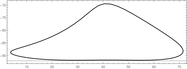
Best regards -- Henrik

POSTED BY: Henrik Schachner

Here a bit nicer with small figures:

enter image description here

And as an animation:

enter image description here

Notebook as attachment. (can now be ran by just executing the entire notebook).

Attachments:
POSTED BY: Sander Huisman

enter image description here - another post of yours has been selected for the Staff Picks group, congratulations !

We are happy to see you at the tops of the "Featured Contributor" board. Thank you for your wonderful contributions, and please keep them coming!

POSTED BY: EDITORIAL BOARD

For 6 pairs of legs (seen in many build-kits), with the phase difference of each successive pairs of legs just being Pi/3, you will get the following animation:

enter image description here

where I marked each pair by number and by F(front) and B(back).

The trajectory of one of the feet can be obtained like so:

pts = Subdivide[0, 2 Pi, 150];
trajectoriesdata = (FindPoints /@ pts)\[Transpose];
trajectoriesdata = trajectoriesdata[[-1]];
Graphics[{Arrow[trajectoriesdata], Point[trajectoriesdata]}, Axes -> True]

enter image description here

To get the angles when it touching we find the minima and maxima in X position:

ClearAll[XPosFeet,XPosFeet2]
XPosFeet[\[Theta]_?NumericQ]:=FindPoints[\[Theta]][[-1,1]]
XPosFeet2[\[Theta]_?NumericQ]:=FindPoints[\[Theta]][[7,1]]
min\[Theta]=\[Theta]/.Quiet@FindMaximum[XPosFeet[\[Theta]],{\[Theta],2,1,3}][[2]];
max\[Theta]=\[Theta]/.Quiet@FindMinimum[XPosFeet[\[Theta]],{\[Theta],4.5,3,6}][[2]];
{min\[Theta]2,max\[Theta]2}={\[Pi]/2+(\[Pi]/2-min\[Theta]),3\[Pi]/2+(3\[Pi]/2-max\[Theta])}

ClearAll[LeftOnGroundQ,RightOnGroundQ]
LeftOnGroundQ[\[Theta]_?NumericQ]:=!(min\[Theta]<Mod[\[Theta],2\[Pi]]<max\[Theta])
RightOnGroundQ[\[Theta]_?NumericQ]:=min\[Theta]2<Mod[\[Theta],2\[Pi]]<max\[Theta]2

Plot[XPosFeet[\[Theta]],{\[Theta],0,2\[Pi]},GridLines->{{min\[Theta],max\[Theta]},{}}]
Plot[XPosFeet2[\[Theta]],{\[Theta],0,2\[Pi]},GridLines->{{\[Pi]/2+(\[Pi]/2-min\[Theta]),3\[Pi]/2+(3\[Pi]/2-max\[Theta])},{}}]
Manipulate[Graphics[{Red,Line[FindLines[\[Theta]]],If[LeftOnGroundQ[\[Theta]],Disk[{-50,-100}],{}],If[RightOnGroundQ[\[Theta]],Disk[{50,-100}],{}]},PlotRange->{{-150,150},{-120,70}},ImageSize->800],{\[Theta],0,2\[Pi]}]

giving:

enter image description here

where the dot now indicates touching.

Now we can do some bigger code to generate a nice diagram:

mp=60;
n=6;
(*\[CurlyPhi]=Table[Mod[5\[Iota],n,1],{\[Iota],1,n}];*)
\[CurlyPhi]=Range[n];
Manipulate[
    Graphics3D[{Darker@Yellow,Table[
        {
        Line[ Map[Prepend[mp \[Iota]],FindLines[\[Theta]+\[CurlyPhi][[\[Iota]]] (2Pi/n)],{2}]],
        {Black,Text[\[Iota],{mp \[Iota],0,50}]}
        },
        {\[Iota],n}
    ]
    ,Black,Line[{{mp 1,0,0},{mp n,0,0}}]
    ,MapThread[Text[#1,{mp (n+1),#2,-100}]&,{{"F","B"},{-50,50}}]
    }
    ,
    Lighting->"Neutral",
    PlotRangePadding->Scaled[.1],
    PlotRange->{{-mp,(n+1)mp},{-150,150},{-150,150}},
    Boxed->False,
    ImageSize->700
    ]
,
{\[Theta],0,2\[Pi]}
]

separators={min\[Theta],max\[Theta],min\[Theta]2,max\[Theta]2};
separators=Table[separators-\[CurlyPhi][[\[Iota]]],{\[Iota],n}];
separators=Mod[Flatten[separators],2\[Pi]];
separators=separators//Prepend[0.0]//Append[2.0\[Pi]];
separators=Union[separators];
regions=Partition[separators,2,1];
expanded=Partition[Subdivide[0,2\[Pi],regions//Length],2,1];

ClearAll[MakeRegionPart]
MakeRegionPart[{\[Theta]start_,\[Theta]stop_},{start_,stop_}]:=Module[{eval,onground,ypos,xpos,pos,support},
    eval=(\[Theta]start+\[Theta]stop)/2.0;
    onground=Table[{LeftOnGroundQ[eval+\[CurlyPhi][[\[Iota]]]],RightOnGroundQ[eval+\[CurlyPhi][[\[Iota]]]]},{\[Iota],n}];
    xpos=Subdivide[start,stop,3][[2;;-2]];
    ypos=Subdivide[0.5,0,n+1][[2;;-2]];
    pos=Partition[Reverse/@Tuples[{ypos,xpos}],2];
    support=MapThread[If[#1,Disk[#2,0.02],{}]&,{onground,pos},2];
    (*Print[support];*)
    {
        Line[{{{\[Theta]start,0.75},{\[Theta]start,1.25}},{{\[Theta]stop,0.75},{\[Theta]stop,1.25}}}],
        Line[{{{start,0},{start,0.5}},{{stop,0},{stop,0.5}}}],
        {Dashed,Opacity[0.5],Line[{{{\[Theta]start,0.75},{start,0.5}},{{\[Theta]stop,0.75},{stop,0.5}}}]},
        support
    }
]

xpos1=Subdivide[Sequence@@expanded[[1]],3][[2;;-2]];
ypos1=Subdivide[0.5,0,n+1][[2;;-2]];

Graphics[{
    MapThread[MakeRegionPart,{regions,expanded}],
    Text[#,{#,1.35}]&/@Range[0,2\[Pi],\[Pi]/2],
    MapThread[Text[#1,{#2,-0.1}]&,{{"F","B"},xpos1}],
    MapThread[Text[#1,{-0.1,#2}]&,{Range[n],ypos1}]
}
]
(*
plts=Table[
Plot[{If[LeftOnGroundQ[\[Theta]+\[CurlyPhi][[\[Iota]]]],20-4\[Iota],Missing[]],If[RightOnGroundQ[\[Theta]+\[CurlyPhi][[\[Iota]]]],20-(4\[Iota]+1),Missing[]]},{\[Theta],0,2\[Pi]}]
,
{\[Iota],n}
];
Show[plts,PlotRange\[Rule]All,GridLines\[Rule]{separators,{}},AspectRatio->1/5,ImageSize\[Rule]1000]*)

Giving:

enter image description here

I attached my notebook so you can change the number of feet and the relative phases between the legs... Note that this notebook was not meant to be easily understood ;-)

Attachments:
POSTED BY: Sander Huisman

@Sander Huisman amazing post! I also would like to point to two demonstrations on the subject, see below. @Marco Thiel, indeed an interesting exciting idea about gait pattern. Sander, do you think we really have to adapt to 12, - is due to instability or inefficiency of this strandbeest with 4 legs? Perhaps it could walk with 4?

Jansen Walker by Contributed by Karl Scherer, Additional contributions: Theo Jansen

A Theo Jansen Walking Linkage by Sándor Kabai

enter image description here

enter image description here

POSTED BY: Vitaliy Kaurov

Indeed an interesting idea, let me see what I can do! These diagrams are made for 2 and 4 legs, i have to adapt it two e.g. 12 legs...

POSTED BY: Sander Huisman

Hi Sander,

very nice indeed! I haven't had the opportunity to run any of this yet - I am on my phone, but I wonder whether it would be interesting to look at the gait pattern with some group theory. Ian Stewart has described such an approach here.

Thanks for posting!

Marco

POSTED BY: Marco Thiel
Reply to this discussion
Community posts can be styled and formatted using the Markdown syntax.
Reply Preview
Attachments
Remove
or Discard