Intro

Languages pack an immense ocean of information, but not only as stories they tell in myths, books, songs, anything we see as the memory of civilization. But also languages are a bottomless well of data related to their structure, relationships, origin, and dynamics of their life and death. In celebration of UNESCO International Mother Language Day (FEB 21) let's see what simple notions we can learn about language diversity using pure data and computation. And here is a spark of thought from UNESCO before we start: "To foster sustainable development, learners must have access to education in their mother tongue and in other languages. It is through the mastery of the first language or mother tongue that the basic skills of reading, writing and numeracy are acquired. Local languages, especially minority and indigenous, transmit cultures, values and traditional knowledge, thus playing an important role in promoting sustainable futures."

Data

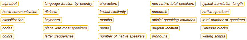
Wolfram Language stores numerous built-in data about natural human languages. We can see it in the following properties:

Multicolumn[EntityProperties["Language"], 5]

There are currently in total 10039 languages in the internal database, which keeps being enriched with data:

langs = EntityList["Language"];
langs // Length

10039

Some languages are dead

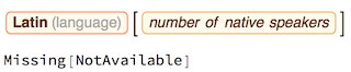
but of course many are not, as you can see right below.

Native speakers

I next compute languages that have number of native speakers listed for them.

popu = DeleteMissing[EntityValue[langs, {"Name", "NativePopulation"}],1, 2];
filt=Select[popu,!StringContainsQ[#[[1]],"script"|"alphabet"]&];
filt//Length

6720

Now I sort languages by native speakers count and show first 100.

barchartPOPU[data_]:=
    BarChart[data,
       ChartLabels->Automatic,
       BarOrigin->Left,
       AspectRatio->2,
       BaseStyle->14,
       PlotTheme->"Business",
       ImageSize->{Automatic,1000},
       ChartStyle->Opacity[.5],
       ChartElementFunction->"GradientScaleRectangle"]

Row[{
    barchartPOPU[Association[Rule@@@SortBy[filt,Last][[-50;;]]]],
    barchartPOPU[Association[Rule@@@SortBy[filt,Last][[-100;;-51]]]]
    }]

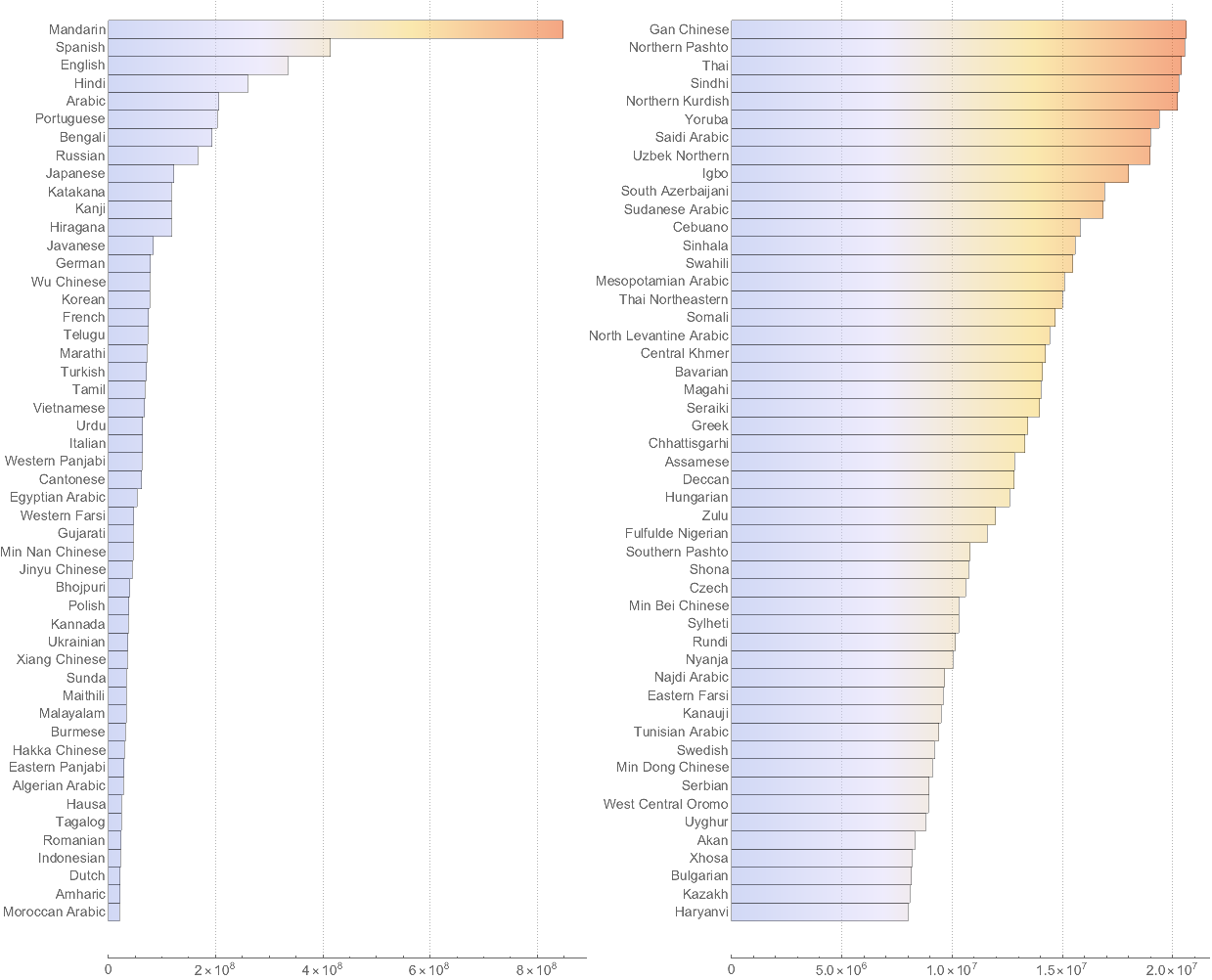
Note, the size of the 1st top bar in the right chart is smaller than the size of the last bottom bar in the left chart - see the axis.

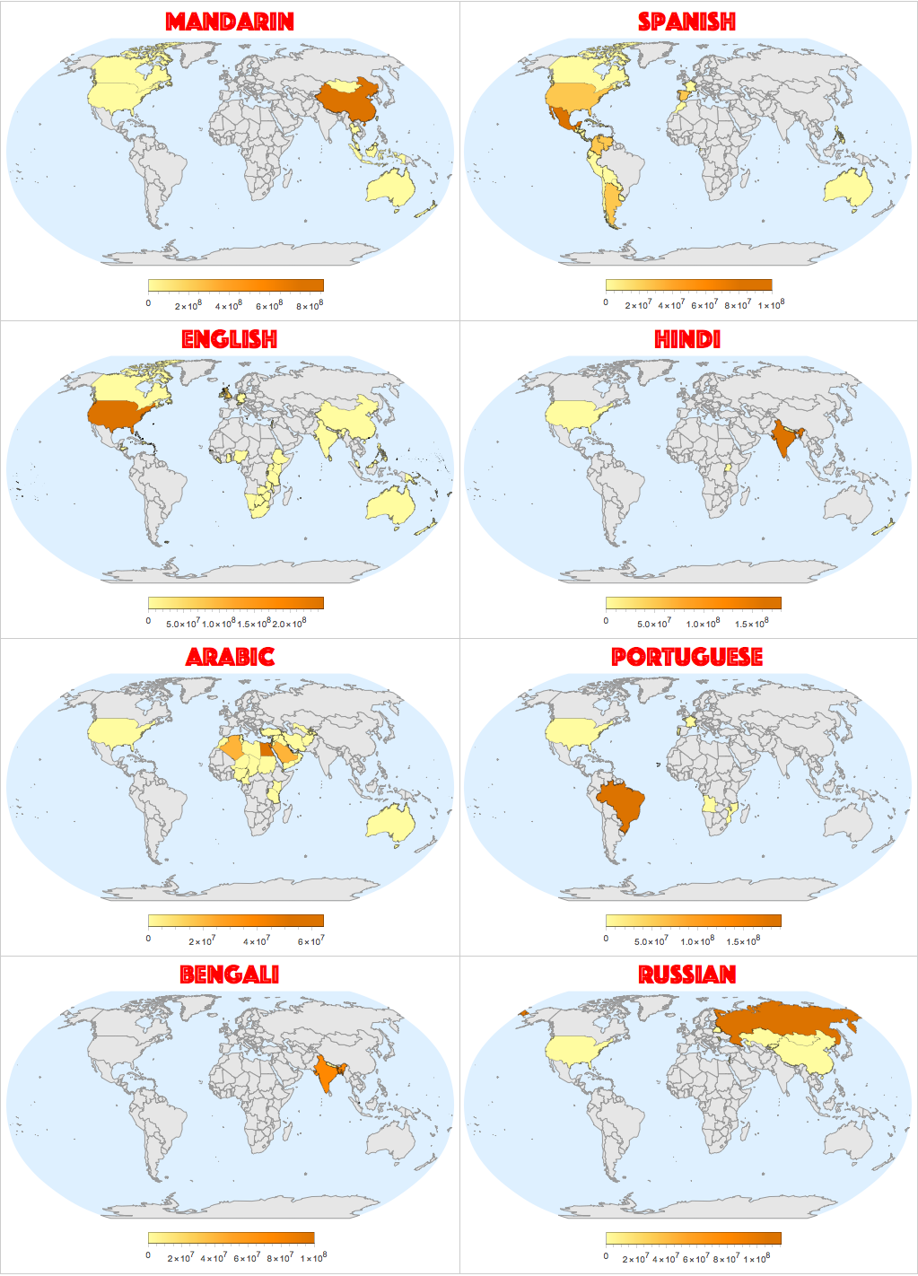
Geographical distribution

One can also learn about how speakers of a specific language are distributed geographically. Let's define a geo-plotting function

geoPLOT[data_,lbl_]:=
GeoRegionValuePlot[data,
    ImageSize->500,
    GeoRange -> "World",
    GeoProjection->"Robinson",
    PlotLabel->Style[lbl,FontFamily->"Phosphate",30,Red],
    GeoBackground ->{"CountryBorders", "Land" -> GrayLevel[.9]},
    PlotLegends->Placed[Automatic,Bottom]
]

and apply it to the first 8 countries with the largest count of native speakers:

Grid[
    Partition[
       geoPLOT@@@EntityValue[Interpreter["Language"][Reverse[SortBy[filt,Last][[-8;;,1]]]],{"Speakers","Name"}]
    ,2],
Frame->All,FrameStyle->GrayLevel[.8]]

Origin and relations

To me the most fascinating data about languages are origin and relations, such as family or lexical similarity. For example let's consider a quite isolated island society of Philippines.

GeoGraphics[
    ({EdgeForm[Red], Opacity[0.1], RandomColor[], Polygon[#1]}&)/@ divisions, ImageSize -> 1000, 
    Epilog -> {Inset[Framed[GeoListPlot[divisions, ImageSize -> 250]], Scaled[{0.85, 0.855}], Automatic], 
    Inset[Framed[GeoGraphics[GeoMarker[Entity["Country", "Philippines"]], 
    GeoRange -> "World", GeoProjection -> "Robinson", ImageSize -> 300]], 
    Scaled[{0.17, 0.93}], Automatic, Scaled[0.4*{1, 1}]]}]

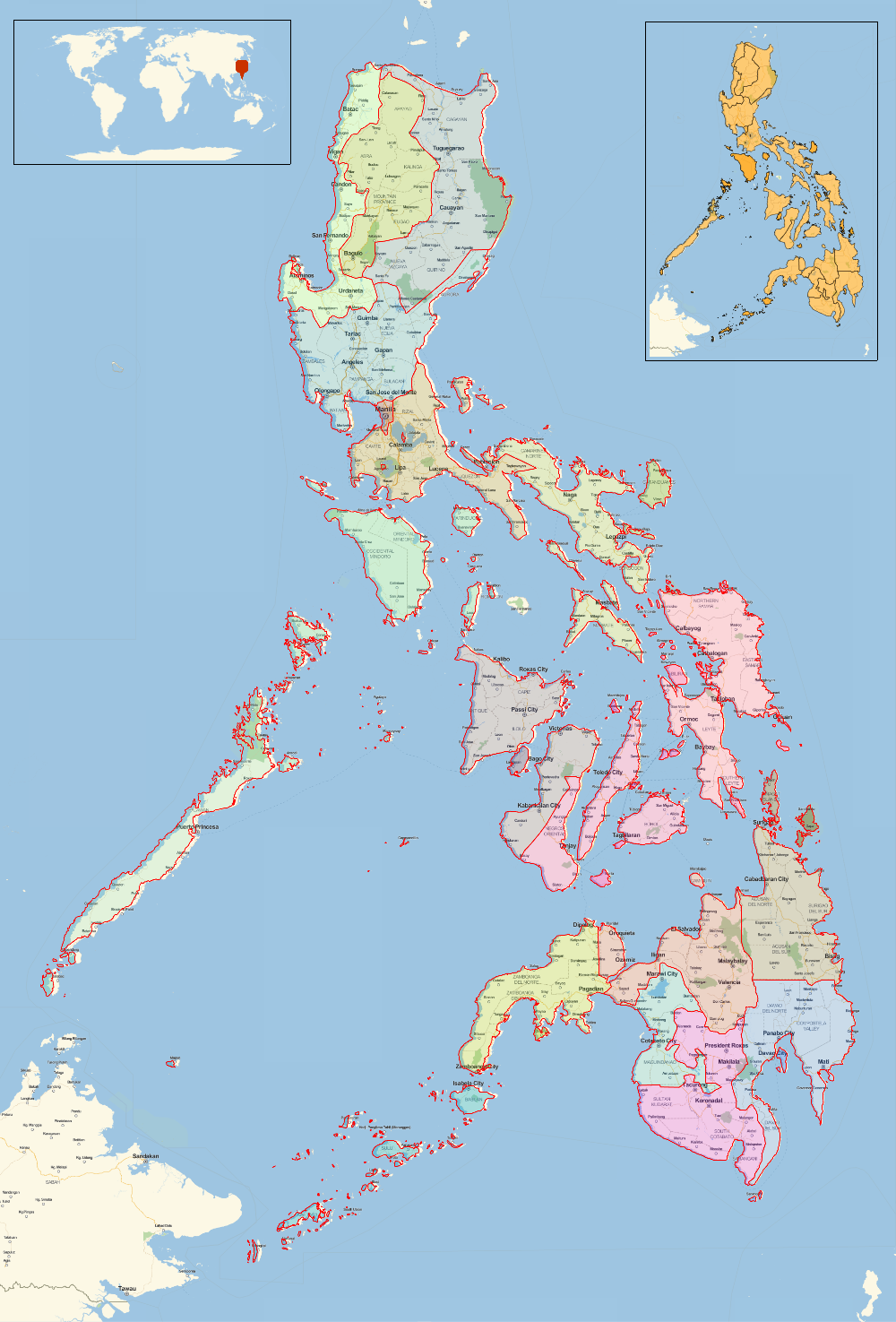
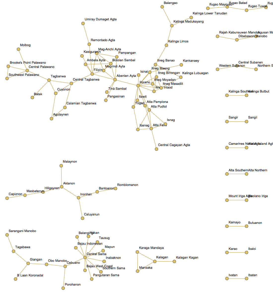
We see above fractured geographic and administrative division structure which perhaps is one of the reasons in past we had formation of complex network of languages. To demonstrate this let's get the data for Lexical Similarity of languages whose Primary Origin is Philippines.

lex=DeleteMissing[EntityValue[langs,{"Name","PrimaryOrigin","LexicalSimilarity"}],1,2];
lex//Length

1092

phil=Cases[lex,{_,Entity["Country", "Philippines"],_}];

I now build a simple network where nodes are languages and an edge exists between any 2 languages having any Lexical Similarity. It is quite fascinating to realize such a complex structure in the same geo-location.

g=Graph[Union[
    Sort/@Flatten[Thread[#1<->#2]&@@@MapAt[CommonName[#[[All,1]]]&,phil[[All,{1,3}]],{All,2}]]
       ],
    VertexLabels->"Name",GraphStyle->"Prototype",
    GraphLayout->"SpringEmbedding",VertexLabelStyle->13,ImageSize->1100]
SetProperty[g,VertexCoordinates->-Reverse/@GraphEmbedding[g]]

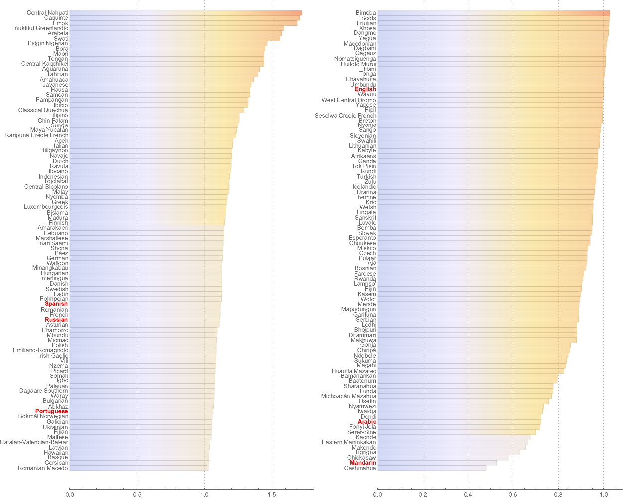
Translation length

Another fun thing to see is typical translation length, which basically tells us do you need more or less characters of a language to express an idea relative to English. We got this info about 180 languages:

trans=DeleteMissing[EntityValue[langs,{"Name","RelativeCharacterCount"}],1,2];
trans//Length

180

We can sort them by translation length and mark in red the top 8 languages with most native speakers shown on the geographic maps above.

Row[{
    barchartPOPU[Association[Rule@@@SortBy[trans,Last][[-90;;]]]],
    barchartPOPU[Association[Rule@@@SortBy[trans,Last][[-180;;-91]]]]
}]/.(#->Style[#,Red,Bold]&/@SortBy[filt,Last][[-8;;,1]])

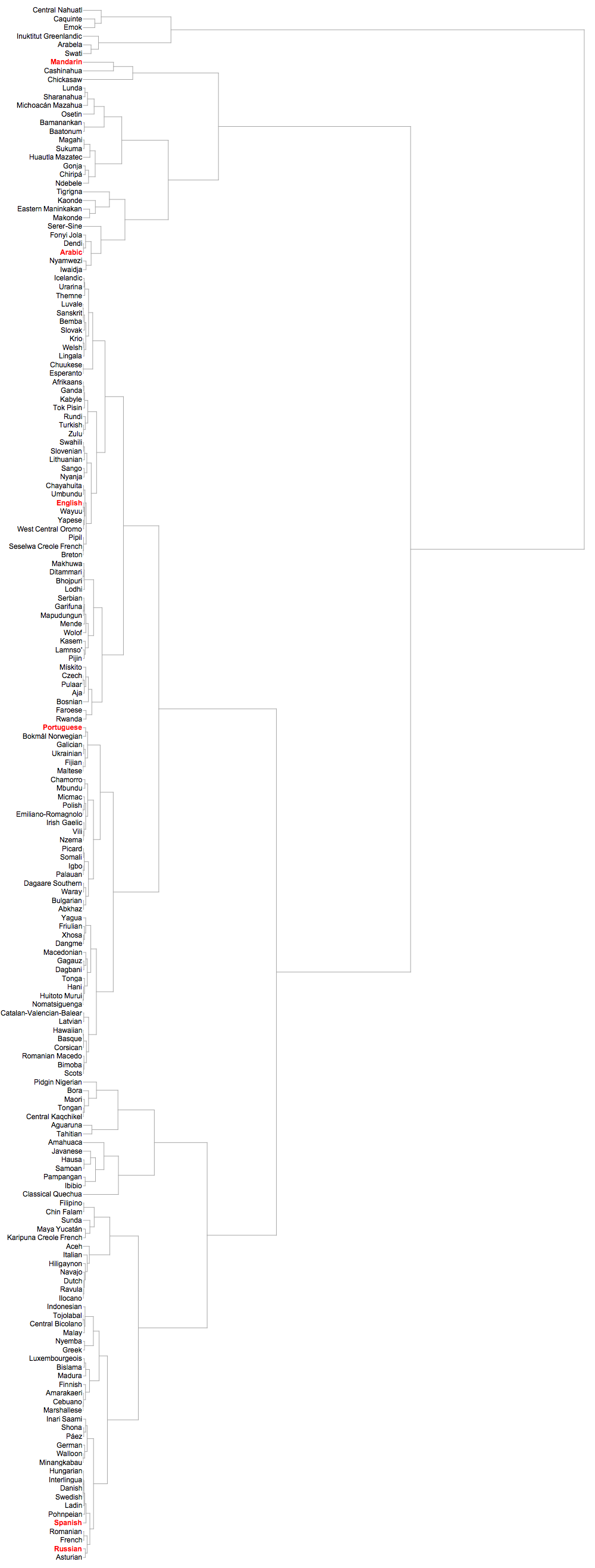
Yet another fun way to look at this is using hierarchical clustering with dendrogram. It helps to group languages by capacity of their writing system to deliver the same information per character sequence length. Again we highlight in red languages with the most native speakers. To me it is amazing to see that English clusters by this property with Wayuu and Umbundu rather with its European friends.

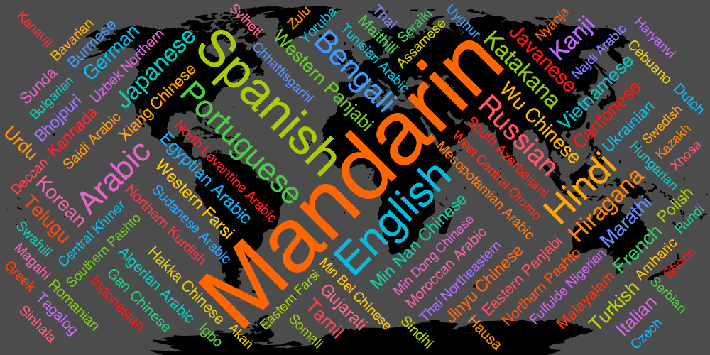
This is where I finish my exploration, but look under the long image below for bonus on how to build the top word cloud overlaid over world map. PLease comment if you can come up with more language related computations and explorations.

Dendrogram[Association[
    Rule@@@Reverse[SortBy[trans,Last]]],
Right,AspectRatio->3,BaseStyle->12,ImageSize->1000,ClusterDissimilarityFunction->"Average"]/.
(#->Style[#,Red,Bold]&/@SortBy[filt,Last][[-8;;,1]])

Bonus

This is how you make the top word cloud overlaid with the world map. The words sizes are scaled by native speaking population.

pl1=GeoGraphics[
    ImageSize->1000,
    AspectRatio->1/2,
    GeoRange -> "World",
    GeoProjection->"Robinson",
    GeoBackground ->{"Coastlines","Land"->Black,"Ocean"->None,"Border"->Black}
];

SeedRandom[2];
pl2=WordCloud[filt,
    AspectRatio->1/2,
    ImageSize->1000,
    WordOrientation->{{-\[Pi]/4,\[Pi]/4}},
    WordSpacings->2,
    PlotTheme->"Marketing"];

Overlay[{pl1, pl2}]