Deformation Animation

Time animation condition: $$ \frac{d}{dt} \Psi \approx \pm c_1, $$ along direction of maximum deformation, $(1,1,1)$. This requires, $$ \frac{d}{dt} E \neq c_2, $$
with arbitrary constants $ c_1, c_2 $.

Color Gradient Surface Tilings

Inspired by Old Veteran Paul Klee Einsame Blute .

To be clear... around 1:00 a.m. 3/7/2017 I did forget to type out the definition of RExp, and later edited it in today.

Temper, ha! My current preference is distemperment. To each his own.

To sum things up, one more point :

• If the built-in functions don't meet user specifications, it's easy for users to code their own improvements using the basic functionality of Mathematica.

Thanks again for your comments, I will keep working on improving the definitions for these algorithms.

Brad

Hi, Danny, thanks for taking some time to respond. I think the code is already out there to satisfy all of your demands, but admittedly I have not been explaining the calculations in any detail. Let's aim for closer to article quality with this post, and see if we can convince ourselves that Mathematica function InverseSeries can be improved on a wide range of inputs. We have not two, but three distinct methods to compare!

Statement of the Problem & Variable Parameters

We start with a power series expansion $$ z = x^m+\sum_{i>m}^{\infty}c_i \; x^i$$ with $m$ defined as the leading power. Without loss of generality we have already assumed that the coefficient of the leading term $c_m$ can be set to $1$ by change of the $x$ variable. We seek a solution $x=f(y(z))$, which expands in whole powers of $y(z)$,

$$ x = y + \sum_{i>1}^{n+1} f_{i}(\mathbf{c}) y^i, $$

with $n$ defined as truncation parameter and $f_{i}(\mathbf{c})$ is in general a complicated, but well structured function of the expansion coefficients $\mathbf{c}= ( c_i:i\in1,2,\ldots )$. It's worthwhile to mention up front that the $f_{i}(\mathbf{c})$ for case $m=1$ have already been explored in numerous outlets including Mathworld, Abramowitz and Stegun, and the OEIS. From the OEIS entry: "The sequence of row lengths is A000041(n) (partition numbers)", which gives us an expectation regarding the number of terms in each $f_i(\mathbf{c})$. This same row-length feature is shared by the triangle for $m=2$, which I added to the OEIS while working on physics problems, including planetary motion, A276738. This is an important feature at any $m$, which we will return to shortly. All functions will take parameters $m$ and $n$ as input and return as output the expansion $x(y(z))$, which inverts the $z(x)$ expansion. Our complexity expectations are as follows:

• Changing $m$ does not change complexity class
• Changing $n$ explores complexity class $\mathcal{O}(p(n))$, where the $p(n)$ are the partition numbers, listed in A000041.

Using the built-in Function

Let's take the code from above MmaExpand, and break it apart into two functions

MmaSeries[n_, m_] := Series[f[x], {x, 0, n + m}] /. 
Join[{f[0] ->  0, (D[f[x], {x, m}] /. x -> 0) -> (m!)}, (D[f[x], {x, #}] /. x -> 0) -> 0 & /@ 
Range[1, m - 1], ((D[f[x], {x, #}] /. x -> 0) -> #! c[#]) & /@ 
Range[m + 1, n + m]]

MmaExpand[n_, m_] := Expand[Refine[Normal[InverseSeries[MmaSeries[n, m]]] /. x -> y^m,  y > 0]]

The first function generates a series and the second function--It's magic to me, slower magic--generates the inverse expansion. Additionally we utilize the small $x$ limit where $z \approx x^m$ to prove that the solution is an expansion in integer powers of $y=z^{1/m}$. This is easy to see once you have studied the multinomial method in the next section. For now we need to run a few critical tests:

AbsoluteTiming[
 RowLengthTest = MatrixForm[Function[{m},
     Length /@ (Coefficient[MmaExpand[8, m], y, #] /. Plus -> List & /@
         Range[3, 8])] /@ Range[5]
   ]]

AbsoluteTiming[ Outer[Coefficient[  Expand[Normal@MmaSeries[4, #1] /. x -> MmaExpand[4, #1]], 
     y, #2] &,  Range[5], Range[5] ] // MatrixForm ]

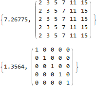
Both are maps where index $m=1,2,3,4,5...$ corresponds to a row. First, we see the number of terms is the partition numbers, as expected. Next in the identity matrix, we see up to power $y^5$ substitution of the inverse series into the series cancels all terms other than $y^m=z$, as required. Let's take for granted that the only problem is time. We obtain timing statistics by mapping over $m$ and $n$

t1=Outer[AbsoluteTiming[MmaExpand[#2, #1]][[1]] &, Range[5], Range[10]]
Out[] = {
{0.00795752, 0.0104603, 0.00681345, 0.00671655, 0.0118878, 0.022436,  0.0632026, 0.159615, 0.443813, 1.42085}, 
{0.00181332, 0.00326319,  0.00738307, 0.0140106, 0.0274177, 0.0521328, 0.118843, 0.26841, 0.684693, 1.9761}, 
{0.00188818, 0.00317625, 0.00734353, 0.013728,   0.0268191, 0.051075, 0.116821, 0.266313, 0.681015,  1.92303}, 
{0.00231411, 0.00382979, 0.0077761, 0.0146602, 0.0272598,  0.0552915, 0.119205, 0.270802, 0.690533, 1.93577},
{0.00201708,  0.00370995, 0.00782772, 0.014608, 0.0296672, 0.0543108, 0.119673, 0.269981, 0.702621, 1.92741}}

We compare these times with other methods.

Multinomial Method

as above:

RExp[n_] := Expand[y Plus[R[0], Total[y^# R[#] & /@ Range[n]]]]
RCalc[0, _] = 1;
RCalc[n_, m_] := With[{basis = Subtract[Tally[Join[Range[n + m], #]][[All, 2]], 
Table[1, {n + m}]] & /@   Select[IntegerPartitions[n + m],    Length[#] > m - 1 &][[2 ;; -1]]}, 
Total@ReplaceAll[    Times[-1/m, Multinomial @@ #, c[Total[#]], 
Times @@ Power[RSet[# - 1] & /@ Range[n + m], #]] & /@     basis, {c[m] -> 1}]]
MultinomialExpand[n_, m_] := (Clear@RSet;   Set[RSet[#], Expand@RCalc[#, m]] & /@ Range[0, n];
Expand[RExp[n] /. R[o_] :> RCalc[o, m]])

The code is a conceptually simple, straightforward realization of the solution method discussed for case $m=2$ in Plane Pendulum and Beyond (rejected by American Journal of Physics), generalized to any $m$. This method is easy to prove, especially for someone versed in ring theory. The algorithm takes advantage of a graded coefficient-algebra associated with partitions of the integer numbers. Rather than writing out a full proof, we can test equivalence:

SameQ[MultinomialExpand[10, #] & /@ Range[5],  MmaExpand[10, #] & /@ Range[5]]
Out[]= True

And now we can run the timing statistics up to $n=18$

t2 = Outer[AbsoluteTiming[MultinomialExpand[#2, #1]][[1]] &, Range[5], Range[18]]
Out[]={{0.000350166, 0.000335676, 0.0006466, 0.00102544, 0.00187701, 
  0.00335827, 0.0050605, 0.00829471, 0.0137534, 0.0213327, 0.0338478, 
  0.0526303, 0.0818673, 0.127584, 0.197492, 0.303197, 0.461779, 
  0.705808}, {0.00059166, 0.000385183, 0.000731424, 0.00141787, 
  0.00256708, 0.00438643, 0.0072424, 0.0121079, 0.0196304, 0.0317456, 
  0.0498247, 0.0797138, 0.123864, 0.19419, 0.297837, 0.463815, 
  0.703707, 1.08945}, {0.000783647, 0.000391522, 0.000853077, 
  0.00165484, 0.00296434, 0.00541067, 0.00877981, 0.0160512, 
  0.0248739, 0.0400204, 0.0637266, 0.101257, 0.158744, 0.247118, 
  0.392642, 0.600964, 0.915037, 1.42288}, {0.000755876, 0.000407823, 
  0.000880547, 0.00177226, 0.0032173, 0.00567963, 0.00968088, 0.01652,
   0.0290402, 0.0468616, 0.0753077, 0.120092, 0.191354, 0.298932, 
  0.466456, 0.734795, 1.09722, 1.70526}, {0.000888697, 0.000464272, 
  0.000976541, 0.00196093, 0.00343374, 0.00653271, 0.0109065, 
  0.0190267, 0.0313326, 0.0523583, 0.0833902, 0.127929, 0.202708, 
  0.327367, 0.512287, 0.798683, 1.23594, 1.91088}}

Still we are under two seconds.

Magic Number Theory Method

as above:

SF[0, 0, m_] = 1;SF[n_, k_, m_] := SF[n, k, m] = 
If[Or[k > n, k < 0], 0,    If[And[n == 0, k == 0], 1, 
SF[n - 1, k - 1, m] + (m*n - 1)*SF[n - 1, k, m]]]
GeneralPolys[n_, m_] :=  MapThread[  Dot, {Table[SF[i, j, m], {i, 0, n - 1}, {j, 0, i}],    
Table[x^j, {i, 0, n - 1}, {j, 0, i}]}]
GeneralT[n_, m_] :=  With[{ps = GeneralPolys[n, m]},   
Table[(-1)^j ps[[j]] /. {x -> i + 2}, {i, 1, n}, {j, 1, i}]]

Basis[n_, m_] :=  Total /@ Map[
Times[m^(-Length[#]) 1/Times @@ (Tally[#][[All, 2]]!), 
Times @@ (# /. x_Integer :> c[x + m])] &, 
Function[{a}, Select[IntegerPartitions[n], Length[#] == a &]] /@ 
Range[n], {2}]

MagicExpand[n_, m_] := Expand[y +   Dot[MapThread[Dot, {GeneralT[n, m], Basis[#, m] & /@ Range[n]}], 
y^Range[2, n + 1]]];

Exploring the expansion coefficients in the OEIS partition triangles A111785 and A276738, I conjectured that it would be possible to store only a regular triangle, i.e., row length equals row index. For example, see: A283247, and triangles for $m=1,2,3...12$ are given in a previous post above. For the final formulation I used Peter Luschny's definitions for the Stirling-Frobenius Cycle numbers . It's conceivable that the above algorithm is easy for a pure mathematician to prove, and also that the above algorithm is already known to someone. I don't know. I found this method by a smart empirical investigation. At this time I can only say that it works, relative to other proven methods, to many orders of magnitude. Here we can check $15$ quickly

SameQ[MagicExpand[15, #] & /@ Range[15],  MultinomialExpand[15, #] & /@ Range[15]]
Out[72]= True

This is a promising result. Although I'm not trained as a mathematician, and mathematicians don't seem to like me very well lately, I'm interested to work on a proof starting from the known algorithm using multinomial coefficients. For now, let's just do the timing test, up to $n=30$

t3 = Outer[AbsoluteTiming[MagicExpand[#2, #1]][[1]] &, Range[5], Range[30]]

Out[75]= {{0.000517401, 0.000730217, 0.00129441, 0.00241826, 
  0.00313761, 0.00480814, 0.00677571, 0.00235547, 0.00322757, 
  0.00458355, 0.00661482, 0.00910492, 0.0127276, 0.0178956, 0.0245657,
   0.03328, 0.045086, 0.0608486, 0.0816343, 0.111034, 0.145875, 
  0.192592, 0.252839, 0.331296, 0.431803, 0.554355, 0.709992, 
  0.907644, 1.15345, 1.45812}, {0.000193195, 0.000157575, 0.000248437,
   0.000478158, 0.000638147, 0.000984389, 0.00152262, 0.00219397, 
  0.00318681, 0.00455035, 0.00642736, 0.00907141, 0.0128466, 
  0.0179599, 0.0244666, 0.0334372, 0.0457468, 0.0618206, 0.0836055, 
  0.115272, 0.151878, 0.196921, 0.259114, 0.338644, 0.436268, 
  0.564819, 0.728962, 0.920223, 1.17813, 1.47938}, {0.000208892, 
  0.000162405, 0.000285868, 0.000402993, 0.000645996, 0.00100673, 
  0.00151145, 0.00223261, 0.00324719, 0.00460649, 0.00675066, 
  0.00924921, 0.0127491, 0.0177939, 0.0250812, 0.0334789, 0.0458992, 
  0.0638416, 0.0865447, 0.112189, 0.149649, 0.198407, 0.25906, 
  0.34008, 0.436906, 0.56552, 0.727684, 0.928567, 1.18617, 
  1.52182}, {0.000167536, 0.000164216, 0.000273794, 0.000405408, 
  0.000670145, 0.000981371, 0.00175083, 0.00223442, 0.00321972, 
  0.00472271, 0.00701268, 0.0105626, 0.0139251, 0.0198001, 0.0275424, 
  0.0371674, 0.0510624, 0.0657576, 0.0853008, 0.120408, 0.156297, 
  0.213033, 0.280924, 0.365606, 0.467034, 0.589213, 0.780763, 1.02078,
   1.23597, 1.59574}, {0.000196817, 0.000165725, 0.000252361, 
  0.000439821, 0.000629393, 0.000999784, 0.00157846, 0.0022308, 
  0.00322183, 0.00483742, 0.00662297, 0.00945479, 0.0128339, 
  0.0181477, 0.0254782, 0.034367, 0.0472682, 0.0632687, 0.0855504, 
  0.113633, 0.152079, 0.201328, 0.268378, 0.346395, 0.478177, 
  0.617492, 0.742203, 0.935041, 1.20908, 1.52182}}

again, under two seconds max time.

Graphing Time Results

Show[
 ListLinePlot[t1,  PlotStyle -> (Blend[{Red, Orange}, #/5] & /@ Range[5]), 
  PlotRange -> All], ListLinePlot[t2, PlotStyle -> (Blend[{Blue, Green}, #/5] & /@ Range[5]), 
  PlotRange -> All],  ListLinePlot[t3, PlotStyle -> Purple, PlotRange -> All], 
 PlotRange -> All, AxesLabel -> {Style["n", 20], Style["t(s)", 20]}, ImageSize -> 800 ]

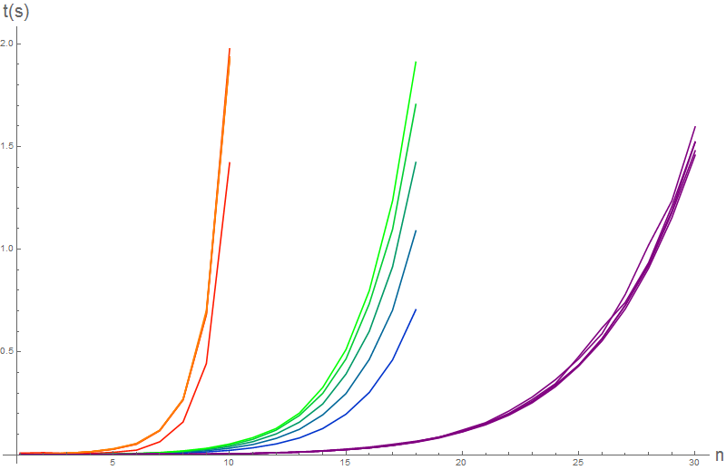
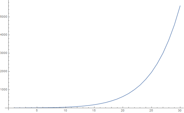
This is the same graph as above, but with extra explanation, maybe it is easier to interpret. As predicted, variation with $m$ is insignificant compared to the blow up with $n$, associated with partition complexity class. Compare with a plot of the partition numbers:

ListLinePlot[Length@IntegerPartitions[#] & /@ Range[20], ImageSize -> 800]

The time graph also shows that in the partition complexity class, regardless of $m$, the magic method vastly outperforms other methods. The easy multinomial method only outperforms the method using built-in inverse function. Setting a time limit of $2s$, we can only compute approximately $10$, $18$, $30$ orders of magnitude, as indexed by $n$.

Again, the most interesting feature of the graph is the stability of the magic method with regard to variation of $m$. If you look closely at the code, tasks seperate into an $\mathcal{O}(n^2)$ listing of coefficients, and an $\mathcal{O}(p(n))$ expansion of functions $g_{i,j}(\mathbf{c})$, called a "basis". Again, if the basis function can be optimized by recursive programming, then the timing can be further reduced.

Danny, does this make more sense? If not maybe we can get a third opinion? Seems like Michael Trott would probably also have some idea about this sort of calculation. Ultimately it would also be interesting to hear from one of you inside the company: How does the Mma algorithm work for inverting a series with symbolic coefficients?

That's all for now,

Brad

Now that I am just talking about numbers and not drawing any pictures, I think this thread may be losing interest. Also we haven't heard from the relevant experts as to why / how I am out-competing a usually-strong Mma function. But I talked breifly with Peter Luschny who found an interesting connection to the Pochammer function. Working from there and searching the OEIS more I obtained the following closed form in terms of MultiFactorial:

MultiFactorial[n_, nDim_] := 
Times[n, If[n - nDim > 1, MultiFactorial[n - nDim, nDim], 1] ]

AlternateGeneralT[n_, nLead_] := 
Table[MultiFactorial[i + nLead j + 2, nLead]/
MultiFactorial[i + 2, nLead], {i, 0, n}, {j, 0, i}] // TableForm

And the following Prints:

Grid[Partition[(Abs@GeneralT[5, #] // TableForm) & /@ Range[12], 4], 
 Frame -> All]

Grid[Partition[AlternateGeneralT[4, #] & /@ Range[12], 4], 
 Frame -> All]

Yield the same triangles

Thank you Wolfram Community Moderation Team, for showing me a little bit of respect.

Conclusion

To reiterate my points:

• What is the Mathematica Algorithm?
• Why is Mathematica going so slow?
• Can we change the Mma Source Code to use one of my definitions or something similar?
• Why aren't any of the triangles above already in OEIS?
• Is this reduction known?

I find the discovery enjoyable, and look forward to finding out just why it works this way. More work ahead . . .

Next, I'm going back to physics research, where I apply these triangles of numbers to perturbation calculations of planetary motion. Furthermore, I have another idea for applying series inversion to make it easy to compute integrals along Rotational Energy Surfaces.

Adapted Multinomial Algorithm

Comparing $n=2$ case above, and $n=1$ case here, it seems like the following simple algorithm could easily be generalized to revert any series with leading term order $n$ :

RExp[n_] := Expand[b Plus[R[0], Total[b^# R[#] & /@ Range[n]]]]
RCalc[n_] := 
With[{basis = Subtract[Tally[Join[Range[n + 1], #]][[All, 2]],
Table[1, {n + 1}]] & /@ IntegerPartitions[n + 1][[2 ;; -1]]},
Total@(Times[-1, Multinomial @@ #, v[Total[#]],
Times @@ Power[RSet[# - 1] & /@ Range[n + 1], #]] & /@ basis)]
InvSeries[n_] := AbsoluteTiming[
Clear@RSet; RSet[0] = 1; 
Set[RSet[#], Expand@RCalc[#]] & /@ Range[n];
Expand[RExp[n] /. R -> RSet]]

Updated Time Test

Conceptually Simple method using multinomial coefficients fits in between slower Mma code and faster unproven method. This is the same time-behavior as seen in the case with leading quadratic term.

Challenge: Calculate series reversion with leading cubic leading term. Is there a regularization of the partition structure? Assuming yes, what is it? How does it relate to results for $n=1,2$ ?