This is a photo of some tree branches that I took at the park today.

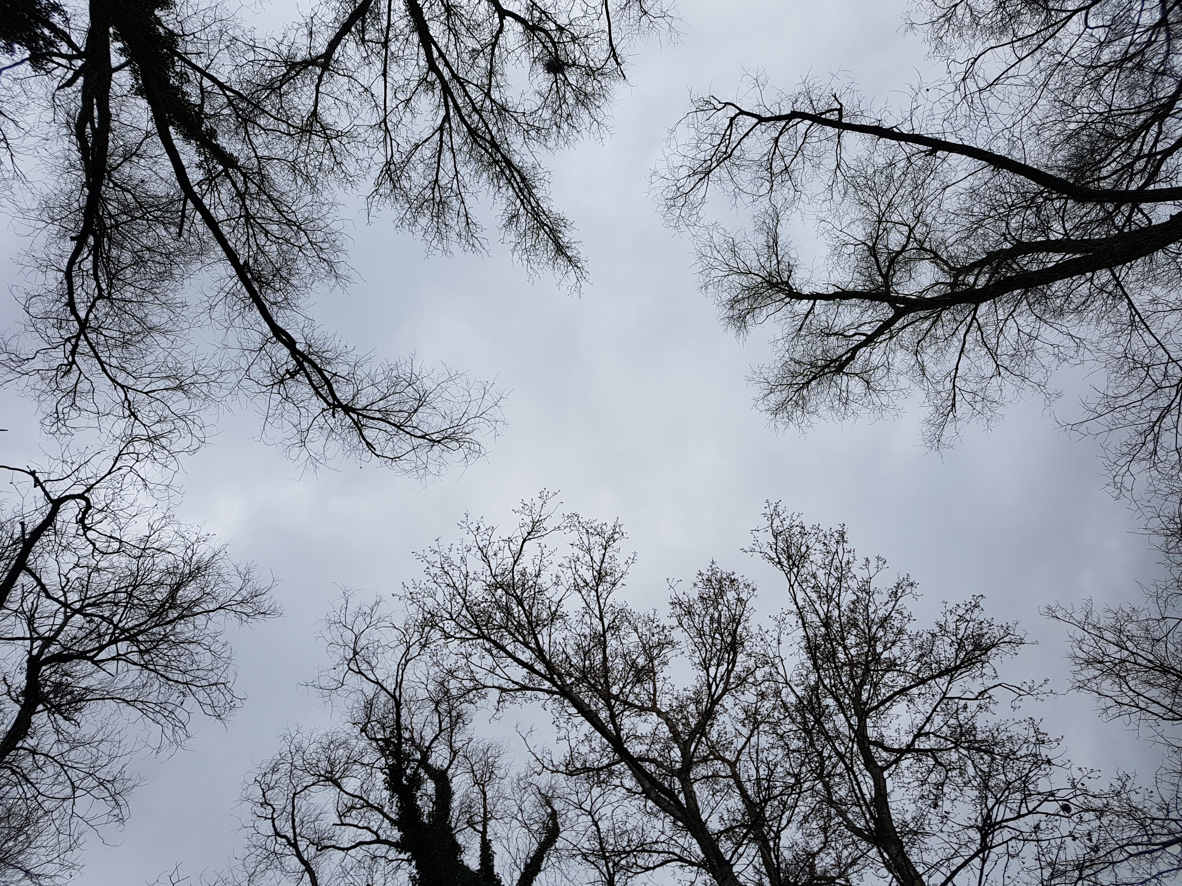
It looks like a fractal, and a nice candidate for measuring the fractal dimension. Here's how we can do that in Mathematica.

Let us start by binarizing the image.

img = Import["~/Downloads/20170304_121322.jpg"];

bin = LocalAdaptiveBinarize[ImageAdjust[img, 0.3], 200, {0.9, 0, 0}];

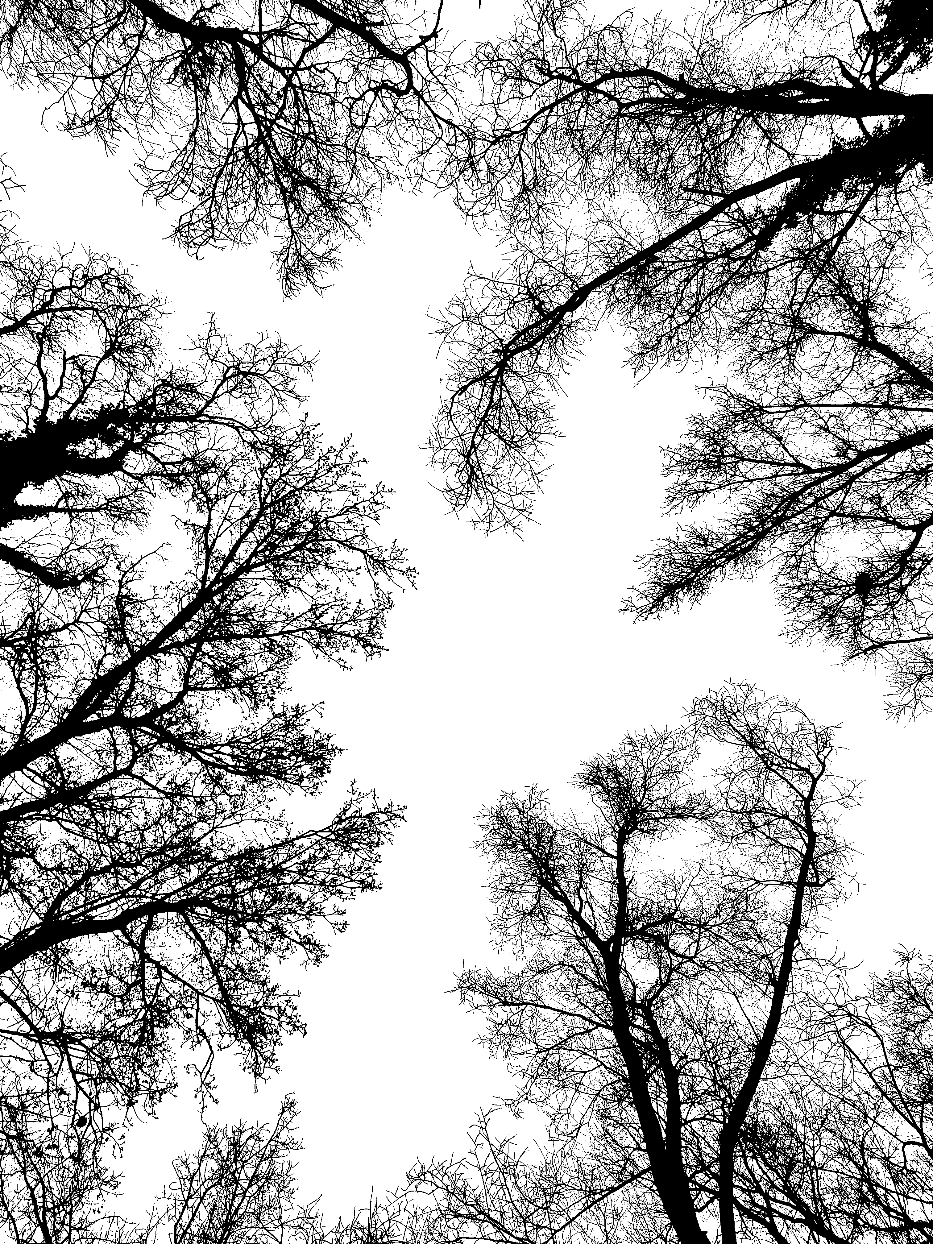
For a better result, I increased the contrast slightly (ImageAdjust), then used local adaptive binarization. This method chooses a different binarization threshold for each pixel based on its neighbourhood. It helps preserve small branches while avoiding including any part of the clouds (the weather was not very good today).

The easiest way to measure fractal dimension is box counting: overlay a square grid, and see how many of the grid cells contain some of the object in the image. What would we get if the object is a line?

Table[
  Rasterize[Graphics[{Antialiasing -> False, Line[{{0, 0}, {1, 1}}]}],
    ImageSize -> 256, RasterSize -> k],
  {k, 2^Range[2, 8]}
  ] // ListAnimate

The box count would double (i.e. multiply by $2^1$) every time the box size is halved. What would happen if the object is a filled disk?

Table[
  Rasterize[Graphics[{Antialiasing -> False, Disk[]}], 
   ImageSize -> 256, RasterSize -> k],
  {k, 2^Range[2, 8]}
  ] // ListAnimate

The box count would quadruple (i.e. multiply by $2^2$) every time the box size is halved.

In general, for a $d$-dimensional object the box count $n$ is proportional to power $-d$ of the box size $l$:   $n \sim l^{-d}$. For some objetcs, $d$ can be a fractional (non-integer) number. Such objects are called fractals. Let's try it on the tree photo!

First, let us choose box sizes in pixels so that an integer number of boxes fit in the image.

seq = Reverse[Intersection @@ Divisors /@ ImageDimensions[img]]
(* {1008, 504, 336, 252, 168, 144, 126, 112, 84, 72, 63, 56, 48, 42, 36, 28, 24, 21, 18, 16, 14, 12, 9, 8, 7, 6, 4, 3, 2, 1} *)

Luckily, the image width and height had many small prime factors in common, so we have many box sizes to work with. Now let us count boxes.

{width, height} = ImageDimensions[img]
(* {3024, 4032} *)

result = {
  width/#,
  Last@First@ImageLevels@Image[
      BlockMap[Min, ImageData[bin], {#, #}],
      "Bit"]
  } & /@ seq; // AbsoluteTiming

(* {9.79212, Null} *)

BlockMap will partition the image data into blocks (i.e. boxes) and take the minimum of each. Since black pixels are represented by 0 and white pixels by 1, we get 0 only for those boxes that contain at least one black pixel, i.e. they contain a bit of the tree branches. BlockMap was introduced in Mathematica 10.2. Those using older versions can substitute BlockMap[f, matrix, {k,k}] by Map[f, Partition[matrix, {k,k}], {2}].

ImageLevels counts how many times each possible pixel value appears in an image. To make sure that the only possible pixel values are 0 and 1, we create a "Bit" image.

Is the result really a power function of the form $n = \text{(const.)} l^d$? The easy way to test this is to plot it on a log-log plot. Power functions appear as a line when plotted on a logarithmic scale.

ListLogLogPlot[result]

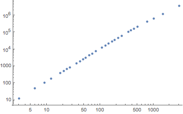
The slope of the line will give the exponent: $\ln n = \ln\text{(const.)} + d \ln l$.

fm = LinearModelFit[Log[result], {1, x}, x]

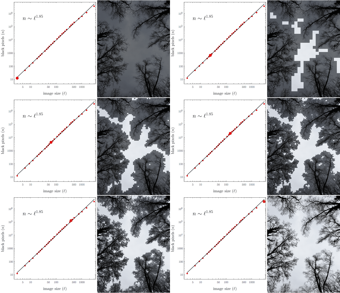
It is about $\approx 1.85$. Despite the thick tree trunks, the image of the branches behaves as a lower-than-two dimensional structure.

Let us plot the power law fit together with the original data:

plot = Show[
  Plot[fm[x], {x, Log[result[[1, 1]]], Log[result[[-1, 1]]]}, 
   PlotStyle -> Black],
  ListLogLogPlot[result, PlotStyle -> Red],
  AspectRatio -> 1, Axes -> False, Frame -> True
  ]

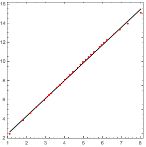
You can see that the power law is a pretty good fit. The slope of the curve is more or less the same at all size scales. This indicates a certain kind of scale invariance in the image. Indeed, it is clear that if we magnified a small part of the image, it would look similar to the whole: small branches are miniature copies of larger ones. This is a characteristic feature of fractals.

To visualize the box counting method, we can show the series of finer and finer box-grids:

sz = 252;
imgs = Image[BlockMap[Min, ImageData[bin], {#, #}], "Bit"] & /@ seq

Scaling them to the same size and animating them show how they approach the original image better and better:

imgs = If[First@ImageDimensions[#] > sz, 
     ImageResize[Image[#, Real], sz], (* downscale as grayscale *)
     ImageResize[#, sz, Resampling -> "Nearest"]] & /@ imgs; (* upscale as bitmap *)

frm = Table[
  ImageCompose[ImageResize[img, 252], {im, 0.5}], {im, imgs}];

ListAnimate[frm]

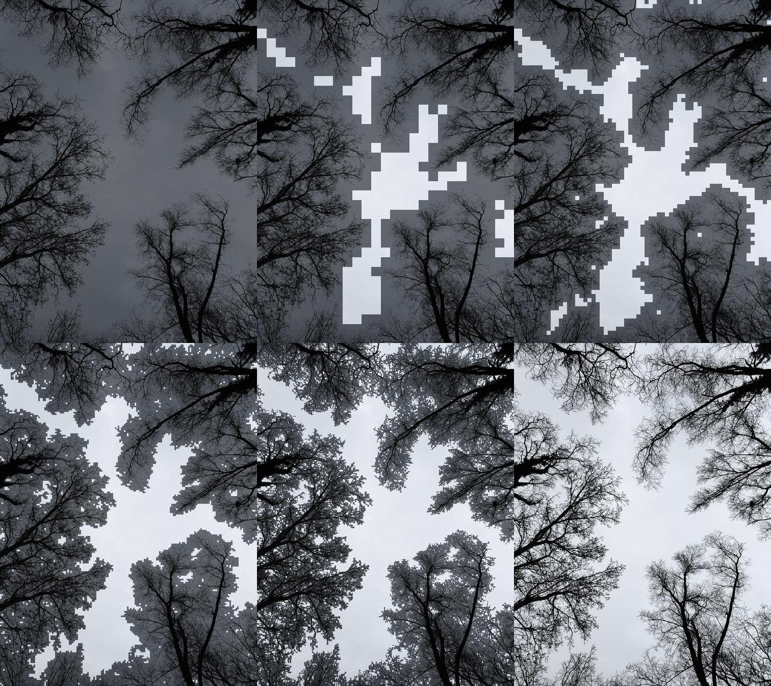
We can show the animation alongside the scaling plot:

frames = Table[
   Row[{
     Show[plot, AspectRatio -> 1, ImageSize -> 336, 
      Epilog -> {AbsolutePointSize[10], Red, Point@Log[result[[i]]]}],
      Image[frm[[i]], Magnification -> 1]
     }],
   {i, Length[imgs]}];

With some extra styling it looks like this:

I hope you enjoyed this small demonstration!