Elliptical Fourier Descriptors for Biological Pattern Recognition

Note: the complete and updated code can be found at: https://github.com/alihashmiii/Elliptical-Fourier-Descriptors

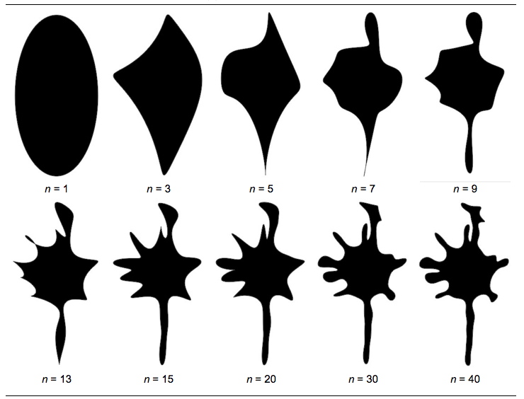
Elliptical Fourier Descriptors is a mathematical technique which utilizes a sum of ellipses over contours to quantify the contours and silhouettes in an image. Broadly speaking the technique is widely used in Computer Vision and visual Pattern Matching. The first mode is by default an ellipse. Even the second or higher harmonics are all ellipses. However when the modes are accumulated we get closer and closer to describing the shape of a given contour.

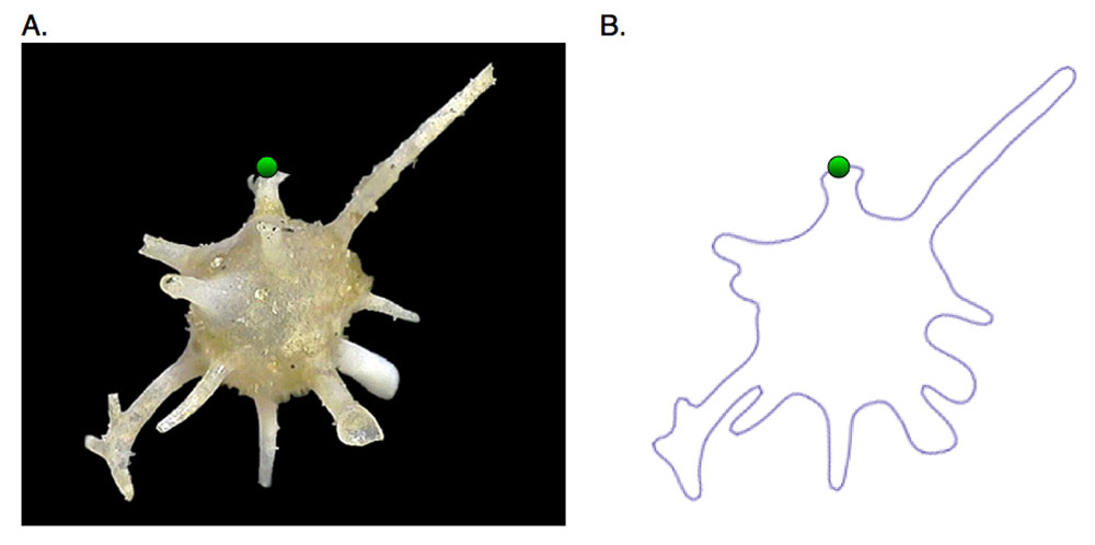
An example might be, say, we are interested in mathematically quantifying a complex shape

Given the image above (courtesy of PalaeoMath) a natural evolution of pattern identification will be as follows:

courtesy of PalaeoMath)

Lately I have been experimenting with aggregates (clusters) of cells that naturally evolve, grow and undergo a change in morphology during their course of development. An attempt to classify the different aggregates is important. It may enable us to understand the mechanical and chemical interactions that determine cell behaviour and fate as a group.

I tried searching for a code in Mathematica (my language of choice) with a robust implementation of Elliptical Fourier Descriptors. Failing to find one I wrote one. The code is a translation from the works of "FEATURE EXTRACTION METHODS FOR CHARACTER RECOGNITION--A SURVEY - OIVIND DUE TRIER et al, Pattern Recognition Vol 29" and also I would like to give credit to Henrik Blidh for a nice Python implementation.

Options[EllipticalFourier] = {normalize -> True, 
   sizeInvariance -> True, order -> 10, ptsToplot -> 300, 
   locus -> {0., 0.}};
EllipticalFourier[img_, OptionsPattern[]] := 
 Module[{dXY, dt, t, T, \[Phi], contourpositions, contour, xi, 
   A0, \[Delta], C0, dCval, coeffL},
  contourpositions = 
   PixelValuePositions[MorphologicalPerimeter[img], 1];
  contour = 
   Part[contourpositions, Last@FindShortestTour[contourpositions]];
  dXY = Differences[contour];
  dt = (x \[Function] N@Sqrt[x])[Total /@ (dXY^2)];
  t = Prepend[Accumulate[dt], 0];
  T = Last@t;
  \[Phi] = 2 \[Pi] t/T;

  normalizeEFD[coeff_] := With[
    {\[Theta] = 
      0.5 ArcTan[(coeff[[1, 1]]^2 - coeff[[1, 2]]^2 + 
          coeff[[1, 3]]^2 - coeff[[1, 4]]^2),
        2 (coeff[[1, 1]] coeff[[1, 2]] + 
           coeff[[1, 3]] coeff[[1, 4]])]},
    Block[{coeffList = coeff, \[Psi], \[Psi]r, a, c, \[Theta]r},
     \[Theta]r[
       i_Integer] := {{Cos[i \[Theta]], -Sin[i \[Theta]]}, {Sin[
         i \[Theta]], Cos[i \[Theta]]}};
     coeffList = Partition[#, 2, 2] & /@ coeffList;
     coeffList = MapIndexed[(#1.\[Theta]r[First@#2]) &, coeffList];
     a = First@Flatten@First@coeffList;
     c = (Flatten@First@coeffList)[[3]];
     \[Psi] = ArcTan[a, c];
     \[Psi]r = {{Cos[\[Psi]], Sin[\[Psi]]}, {-Sin[\[Psi]], 
        Cos[\[Psi]]}};
     coeffList = MapIndexed[Flatten[\[Psi]r.#] &, coeffList];
     If[OptionValue[sizeInvariance], a = First@First@coeffList; 
      coeffList /= a, coeffList]]
    ];

  ellipticalCoefficients[order_] := Module[{coeffs, func},
    func[list : {{__} ..}, n_Integer] := 
     Block[{listtemp = list, const = T/(2 (n^2) ( \[Pi]^2)), 
       phiN = \[Phi] *n,
       dCosPhiN, dSinPhiN, an, bn, cn, dn},
      dCosPhiN = Cos[Rest@phiN] - Cos[Most@phiN];
      dSinPhiN = Sin[Rest@phiN] - Sin[Most@phiN];
      an = const*Total@(dXY[[All, 1]]/dt *dCosPhiN);
      bn = const*Total@(dXY[[All, 1]]/dt*dSinPhiN);
      cn = const*Total@(dXY[[All, 2]]/dt*dCosPhiN);
      dn = const*Total@(dXY[[All, 2]]/dt*dSinPhiN);
      listtemp[[n]] = {an, bn, cn, dn};
      listtemp
      ];
    coeffs = ConstantArray[0, {order, 4}];
    coeffL = 
     If[OptionValue@normalize, normalizeEFD[#], #] &@
      Fold[func, coeffs, Range@order]
    ];

  dcCoefficients := (
    xi =  Accumulate[Part[dXY, All, 1]] - (dXY[[All, 1]]/dt)*Rest@t;
    A0 = (1/T)*
      Total@(dXY[[All, 1]]/(2 dt) * Differences[t^2] +  xi*dt);
    \[Delta] = 
     Accumulate[Part[dXY, All, 2]] - (dXY[[All, 2]]/dt)*Rest@t;
    C0 = (1/T)*
      Total@(dXY[[All, 2]]/(2 dt) * Differences[t^2] +  \[Delta]*dt);
    {First@First@contour + A0, Last@First@contour + C0}
    );

  plotEFD[coeff_] := 
   Last@Reap@Block[{n = Length@coeff, nhalf, nrow = 2, ti,
       xt, yt, func, \[Theta], i = OptionValue[ptsToplot]},
      nhalf = Ceiling[n/2];
      ti = Array[# &, i, {0., 1}];
      xt = ConstantArray[OptionValue[locus][[1]], i];
      yt = ConstantArray[OptionValue[locus][[2]], i];
      Do[
       xt += 
        coeff[[j, 1]] Cos[2 (j) \[Pi] ti] + 
         coeff[[j, 2]] Sin[2 (j) \[Pi] ti];
       yt += 
        coeff[[j, 3]] Cos[2 (j) \[Pi] ti] + 
         coeff[[j, 4]] Sin[2 (j) \[Pi] ti];
       Sow@
        Graphics[{{Thick, XYZColor[0, 0, 1, 0.8], 
           Line@contour}, {Thick, XYZColor[1, 0, 0, 0.6], 
           Line@Thread[{xt, yt}]}, 
          Inset[Style[#, Bold, Darker@Green, FontSize -> 12] &@
            Text["Harmonic: " <> ToString@j]]}];
       , {j, 1, Length@coeff}];
      ];

  ellipticalCoefficients[OptionValue[order]];
  plotEFD[coeffL]
  ]

The code is initialized as follows:

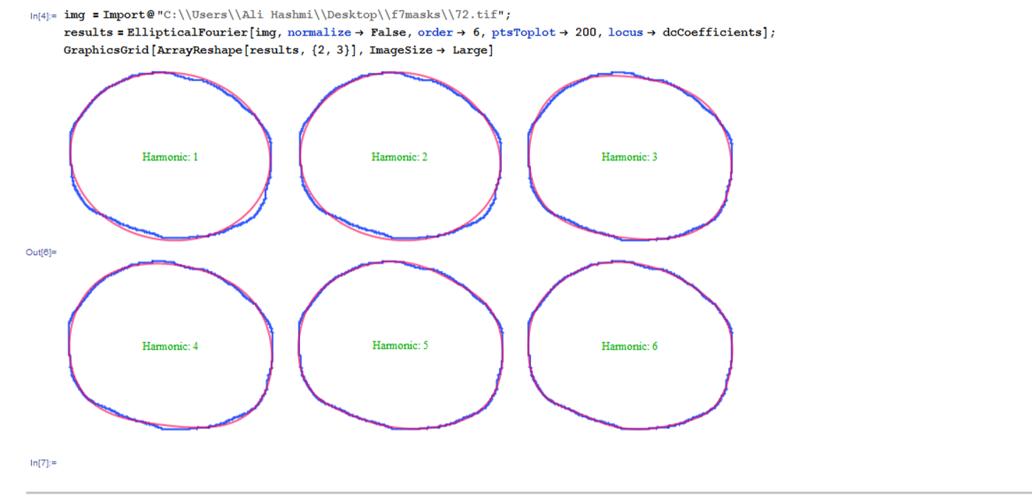
img = Import@"C:\\Users\\Ali Hashmi\\Desktop\\f7masks\\72.tif";
results = 
  EllipticalFourier[img, normalize -> False, order -> 6, 
   ptsToplot -> 200, locus -> dcCoefficients];
GraphicsGrid[ArrayReshape[results, {2, 3}], ImageSize -> Large]

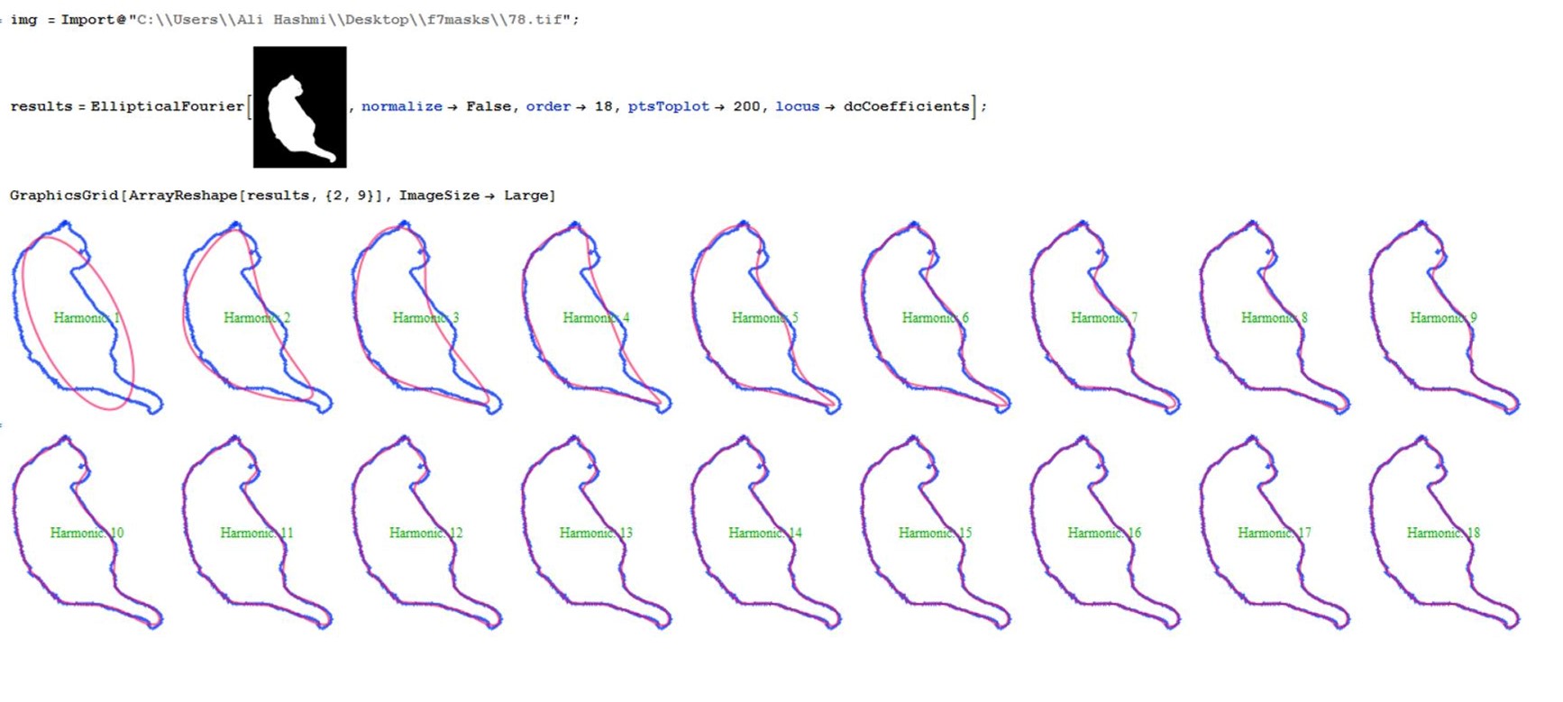
A couple of tests were performed and the results can be seen below:

It is quite evident that the red curve tends to converge toward the blue curve (cat) as the harmonics get higher. In essence the more convoluted the shape, the higher the number of harmonics required to describe the shape.

I also happened to test them on my aggregates and the results look good.

Next I will try to use the shape descriptors to quantitatively analyze the cell clusters

Attachments: