Okay S.B. is officially over, so what am I even doing still theorizing about Alien writing systems? No one knows for sure. Maybe in an obtuse way, it's another dissertation topic in the making. One more discovery to write out, then hopefully I will get back to more mundane, professionally acceptable activities.
Part N. Approximating and Inscribing the Schwarz P Surface
The Schwarz Minimal Surface, P for Primitive, is simple and symmetrical, perhaps a better starting place than the Gyroid. A common approximation is given by:
$$\cos(x)+\cos(y)+\cos(z)=0,$$
but this is wrong, and goes against the definition provided by Lagrange's equation above. Discrepancies, including another
$r^5$ problem, become apparent when subjecting the trial function to due scrutiny. As above, start by rotating coordinates and solving for height along the surface normal,
ApproxP = Sin[x] + Cos[y - Pi/2] + Sin[w];
ApproxP2 =   ApproxP /.   MapThread[
Rule, {{x, y, w},  RotationMatrix[{{0, 0, 1}, {1, 1, 1}}].{x, y, w}}];

ContourF =   Normal[Series[
Normal[InverseSeries[Series[ApproxP2, {w, 0, 5}], k]] /. {k -> 0,
x -> \[Rho] Cos[\[Phi]], y -> \[Rho] Sin[\[Phi]]}, {\[Rho], 0, 5}]];
Expand[TrigReduce[ContourF]]
ContourFxy  =  Expand[ContourF /. {Cos[\[Phi]] -> x/\[Rho],
Sin[\[Phi]] -> y/\[Rho]}]

This expansion provides a baseline for comparison. Again define expansion variables, this time a pair with dihedral-3 symmetry,
r = Sqrt[x^2 + y^2]; P = y/r; Q = x/r;
Q3 = 4 Q^3 - 3 Q; P3 = 3 P - 4 P^3;
g3 = Expand[r^3 Q3 ];
g2 = x^2 + y^2.
Then generate expansion primitives up to a large order, say
$21$,
indList[n_] :=  Select[IntegerPartitions[n],
  MemberQ[{{2, 3}, {2}, {3}}, Union[#]] &]
coeff[ind_] :=  c @@ Flatten[{Cases[Tally[ind], {2, x_} :> x],
     Cases[Tally[ind], {3, x_} :> x]} /. {} -> 0]
params = Flatten[indList[#] & /@ Range[2, 21], 1];
Expand and cancel terms order-by-order
\[CapitalPsi] =   Expand[Total[(coeff[#] Times @@ (# /. {2 -> g2, 3 -> g3})) & /@   params]];
MeanCurvatureNumerator[F_] := Expand[((1 + D[F, x]^2)*D[F, {y, 2}] -
2 D[F, x] *D[F, y] *D[D[F, y], x] + (1 + D[F, y]^2)*D[F, {x, 2}])]

AbsoluteTiming[ CurvExp = Expand[MeanCurvatureNumerator[\[CapitalPsi]]]; ] (*10(s)*)

Sols[n_] :=  Fold[Join[#1, Expand@Solve[#2[[2]] /. #1 , #2[[1]]][[1]]] &, {},
Transpose[{(coeff /@ indList[2 + #]) & /@ Range[0, n],
Function[{a}, # == 0 & /@ (Coefficient[Coefficient[CurvExp, x, #], y,
a - #] & /@ Range[0, a])][#] & /@ (Range[0, n])}] ] // Quiet

AbsoluteTiming[ S19 = Sols[19];]
The first thing to check is:
In[]:= S19[[3]]
Out[]= c[1, 1] -> 0
According to the convention for coefficients,
$c_{1,1}$ attaches to the only
$r^5$ term, so again, a dihedral-3 surface patch cannot have an
$r^5$ term and also satisfy the zero curvature condition. The next check is for degrees of freedom
Length@indList[#] & /@ Range[21]
Subtract[%,  Range[21] /. Append[Rule @@ # & /@
Tally[S19[[All, 1]] /. c[x_, y_] :> 2 x + 3 y], x_Integer :> 0]]
Out[] = {0, 1, 1, 1, 1, 2, 1, 2, 2, 2, 2, 3, 2, 3, 3, 3, 3, 4, 3, 4, 4}
Out[] = {0, 0, 1, 0, 0, 1, 0, 0, 1, 0, 0, 1, 0, 0, 1, 0, 0, 1, 0, 0, 1}
This is an intriguing reduction, that seems to imply the degrees of freedom are enough for any boundary that expands in terms
$\cos(3nx)$, even implying that this method could lead to an exact solution. But our solution today is only "fast richtig", and rather than suffering over the boundary conditions too much, we simply set
$c_{n,m}=1/(2n+3m)!$, to force convergence in a small region around the expansion point, quickly!
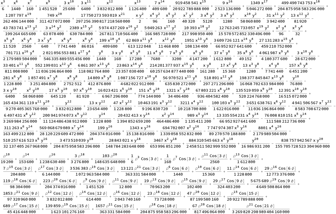
\[CapitalPsi]19 = \[CapitalPsi] //. S19 /.   c[x_, y_] :> 1/(2 x + 3 y)!
TrigReduce[\[CapitalPsi]19 /. {x -> \[Rho] Cos[\[Phi]],  y -> \[Rho] Sin[\[Phi]]}]

Next, compare the curvature
MeanCurvature[F_] := Divide[
Expand[((1 + D[F, x]^2)*D[F, {y, 2}] -
2 D[F, x] *D[F, y] *D[D[F, y], x] + (1 + D[F, y]^2)*
D[F, {x, 2}])],  (1 + D[F, x]^2 + D[F, y]^2)^(3/2)]

curv1 = MeanCurvature[ContourFxy];
curv2 = MeanCurvature[\[CapitalPsi] //. S19 /. c[x_, y_] :> 1/(2 x + 3 y)!];

Row[{Plot3D[{curv1, curv2}, {y, -7/5, 7/5}, {x, -7/5, 7/5},
PlotRange -> All,    RegionFunction -> Function[{x, y, z}, x^2 + y^2 <= (6/5)^2],
ImageSize -> 400],
Plot3D[{curv1, curv2}, {y, -7/5, 7/5}, {x, -7/5, 7/5},    PlotRange -> All,
RegionFunction -> Function[{x, y, z}, x^2 + y^2 <= (7/5)^2],
ImageSize -> 400]}]
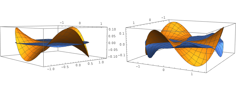
 The left image, up to
$r=6/5$ shows approximately zero curvature for the
$\Psi$ expansion, along the flat blue disk, compared with values about
$0.1$ for the common expansion, depicted as a warped orange disk. In the right image, breakdown of the approximation begins to show at
$r = 7/5$, which sets an outermost boundary. Yet the approximation
$\Psi$ still seems considerably better than the simple approximation.
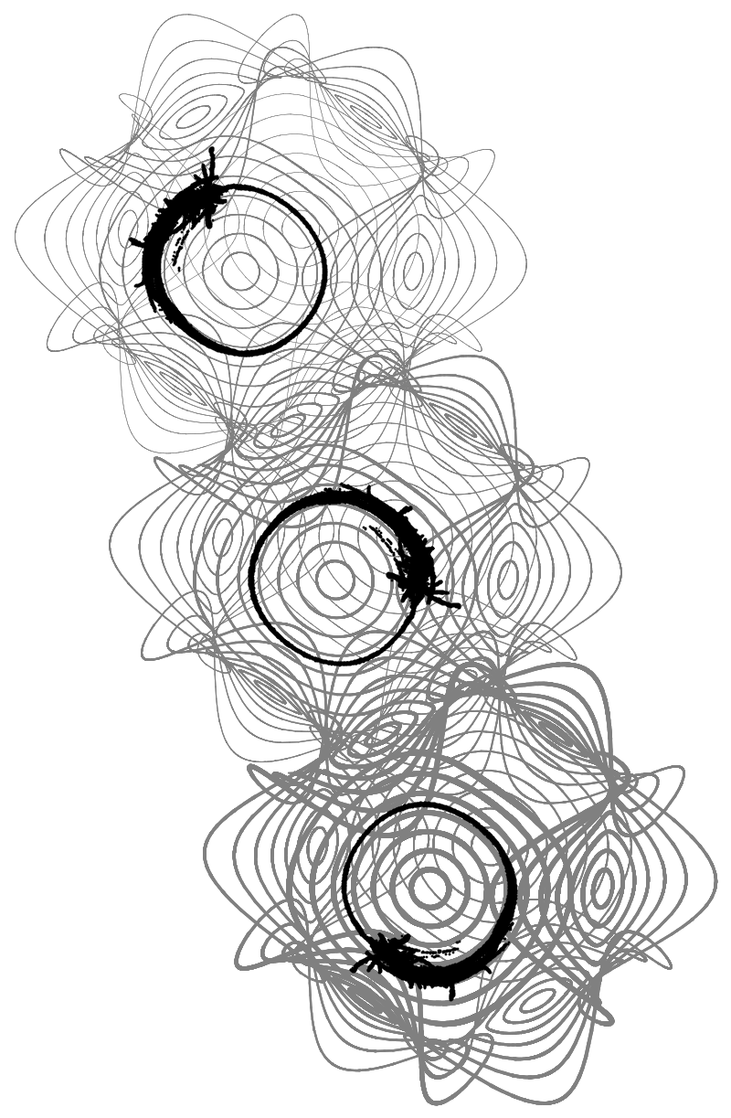
This is all the groundwork we need, the rest is simply extension of the code above. The results,

When I have more time and peace of mind, I will see if I can figure out the boundary conditions. As for now they look good enough by guesswork. I don't know the thing about Weierstrass parameters, I probably never will ! More code here .