I recently watched "Arrival", and thought that some of the dialogue sounded Wolfram-esque. Later, I saw the following blog post:

Quick, How Might the Alien Spacecraft Work?

Along with many others, I enjoyed the movie. The underlying artistic concept for the alien language reminded me of decade old memories, a book by Stephen Addiss, Art of Zen. Asian-influenced symbolism is an interesting place to start building a sci-fi concept, even for western audiences.

I also found Cristopher Wolfram's broadcast and the associated files:

Youtube Broadcast

Github Files ( with image files )

Thanks for sharing! More science fiction, yes!

I think the constraint of circular logograms could be loosened. This leads to interesting connections with theory of functions, which I think the Aliens would probably know about.

The following code takes an alien logogram as input and outputs a deformation according to do-it-yourself formulation of the Pendulum Elliptic Functions:

$m=2$ Inversion Coefficients

MultiFactorial[n_, nDim_] := Times[n, If[n - nDim > 1, MultiFactorial[n - nDim, nDim], 1]]
GeneralT[n_, m_] :=  Table[(-m)^(-j) MultiFactorial[i + m (j - 1) + 1, m]/ MultiFactorial[i + 1, m], {i, 1, n}, {j, 1, i}]
a[n_] := With[{gt = GeneralT[2 n, 2]}, gt[[2 #, Range[#]]] & /@ Range[n] ]

Pendulum Values : $2(1-\cos(x))$ Expansion Coefficients

c[n_ /; OddQ[n]] := c[n] = 0;
c[n_ /; EvenQ[n]] := c[n] = 2 (n!) (-2)^(n/2)/(n + 2)!;

Partial Bell Polynomials

Note: These polynomials are essentially the same as the "BellY" ( hilarious naming convention), but recursion optimized. See timing tests below.

B2[0, 0] = 1;
B2[n_ /; n > 0, 0] := 0;
B2[0, k_ /; k > 0] := 0;
B2[n_ /; n > 0, k_ /; k > 0] := B2[n, k] = Total[
    Binomial[n - 1, # - 1] c[#] B2[n - #, k - 1] & /@ 
     Range[1, n - k + 1] ];

Function Construction

BasisT[n_] :=  Table[B2[i, j]/(i!) Q^(i + 2 j), {i, 2, 2 n, 2}, {j, 1, i/2}]
PhaseSpaceExpansion[n_] :=   Times[Sqrt[2 \[Alpha]], 1 + Dot[MapThread[Dot, {BasisT[n], a[n]}], (2 \[Alpha])^Range[n]]];
AbsoluteTiming[CES50 = PhaseSpaceExpansion[50];] (* faster than 2(s) *)
Fast50 = Compile[{{\[Alpha], _Real}, {Q, _Real}}, Evaluate@CES50];

Image Processing

note: This method is a hack from ".jpg" to sort-of vector drawing. I haven't tested V11.1 vectorization functionality, but it seems like this could be a means to process all jpg's and output a file of vector polygons. Anyone ?

LogogramData = Import["Human1.jpg"];
Logogram01 = ImageData[ColorNegate@Binarize[LogogramData, .9]];
ArrayPlot@Logogram01;

Positions1 = 
  Position[Logogram01[[5 Range[3300/5], 5 Range[3300/5]]], 1];
Graphics[{Disk[#, 1.5] & /@ Positions1, Red, 
   Disk[{3300/5/2, 3300/5/2}, 10]}];
onePosCentered = 
  N[With[{cent = {3300/5/2, 3300/5/2} }, # - cent & /@ Positions1]];
radii = Norm /@ onePosCentered;
maxR = Max@radii;
normRadii = radii/maxR;
angles = ArcTan[#[[2]], #[[1]]] & /@ onePosCentered;
Qs = Cos /@ angles;

Constructing and Printing Image Frames

AlienWavefunction[R_, pixel_, normRad_, Qs_, angles_] := Module[{
   deformedRadii = MapThread[Fast50, {R normRad, Qs}],
   deformedVectors = Map[N[{Cos[#], Sin[#]}] &, angles],
   deformedCoords
   },
  deformedCoords = 
   MapThread[Times, {deformedRadii, deformedVectors}];
  Show[ PolarPlot[ Evaluate[
     CES50 /. {Q -> Cos[\[Phi]], \[Alpha] -> #/10} & /@ 
      Range[9]], {\[Phi], 0, 2 Pi}, Axes -> False, 
    PlotStyle -> Gray],
   Graphics[Disk[#, pixel] & /@ deformedCoords], ImageSize -> 500]]

AbsoluteTiming[  OneFrame = 
   AlienWavefunction[1, (1 + 1)* 1.5/maxR, normRadii, Qs, angles]
 ](* about 2.5 (s)*)

Validation and Timing

In this code, we're using the magic algorithm to get up to about $100$ orders of magnitude in the half energy, $50$ in the energy. I did prove $m=1$ is equivalent to other published forms, but haven't found anything in the literature about $m=2$, and think that the proving will take more time, effort, and insight (?). For applications, we just race ahead without worrying too much, but do check with standard, known expansions:

EK50 = Normal@ Series[D[ Expand[CES50^2/2] /.  Q^n_ :> (1/2)^n Binomial[n, n/2], \[Alpha]], {\[Alpha], 0, 50}];
SameQ[Normal@  Series[(2/Pi) EllipticK[\[Alpha]], {\[Alpha], 0, 50}], EK50]
Plot[{(2/Pi) EllipticK[\[Alpha]], EK50}, {\[Alpha], .9, 1}, ImageSize -> 500]
Out[]:= True

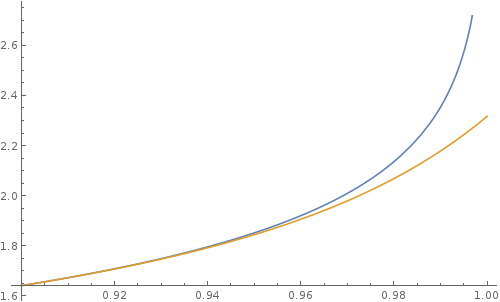
This plot gives an idea of approximation validity via the time integral over $2\pi$ radians in phase space. Essentially, even the time converges up to, say, $\alpha = 0.92$. Most of the divergence is tied up in the critical point, which is difficult to notice in the phase space drawings above.

Also compare the time of function evaluation:

tDIY = Mean[ AbsoluteTiming[Fast50[.9, RandomReal[{0, 1}]] ][[1]] & /@ Range[10000]];
tMma = Mean[AbsoluteTiming[JacobiSN[.9, RandomReal[{0, 1}]] ][[1]] & /@ Range[10000]];
tMma/tDIY

In the region of sufficient convergence, Mathematica function JacobiSN is almost 20 times slower. The CES radius also requires a function call to JacobiCN, so an output-equivalent AlienWavefunction algorithm using built-in Mathematica functions would probably take at least 20 times as long to produce. When computing hundreds of images this is a noticeable slow down, something to avoid ! !

Also compare time to evaluate the functional basis via the Bell Polynomials:

 BasisT2[n_] := Table[BellY[i, j, c /@ Range[2 n]]/(i!) Q^(i + 2 j), {i, 2, 2 n,  2}, {j, 1, i/2}];
SameQ[BasisT2[20], BasisT[20]]
t1 = AbsoluteTiming[BasisT[#];][[1]] & /@ Range[100];
t2 = AbsoluteTiming[BasisT2[#];][[1]] & /@ Range[25];
ListLinePlot[{t1, t2}, ImageSize -> 500]

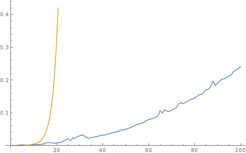
The graph shows quite clearly that careful evaluation via the recursion relations changes the complexity of the inversion algorithm to polynomial time, $(n^2)$, in one special example where the forward series expansions coefficients have known, numeric values.

Conclusion

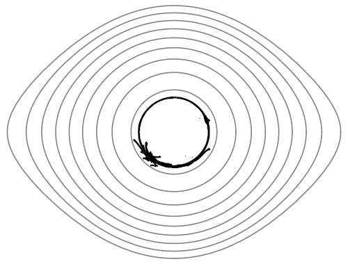
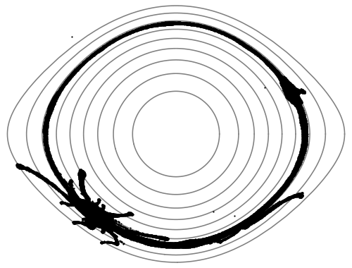
We show proof-of-concept that alien logograms admit deformations that preserve the cycle topology. Furthermore we provide an example calculation where the "human" logogram couples to a surface. Deformation corresponds to scale transformation of the logogram along the surface. Each deformation associates with an energy.

Invoking the pendulum analogy gives the energy a physical meaning in terms of gravity, but we are not limited to classical examples alone. The idea extends to arbitrary surfaces in two, three or four dimensions, as long as the surfaces have local extrema. Around the extrema, there will exist cycle contours, which we can inscript with the Alien logograms. This procedure leads readily to large form compositions, especially if the surface has many extrema. Beyond Fourier methods, we might also apply spherical harmonics, and hyperspherical harmonics to get around the limitation of planarity.

The missing proof... Maybe later. LOL! ~ ~ ~ ~ Brad

And in the Fanfiction Voice:

Physicist : "It should be no surprise that heptapod speech mechanism involves an arbitrary deformation of the spacetime manifold."

Linguist : "Space-traveling aliens, yes, of course they know math and physics, but Buddhist symbology, where'd they learn that?"