Introduction
Perhaps there are already Mma-Procedures to calculate NMR-spectra, but I did not do a literature research.
I post a notebook to calculate NMR-Spectra of simple spin I = 1/2 systems.
The notebook comes in two parts.
Part one uses a spin-product function approach, where the spin-product function a, a ,...b is used as e.g. phi [ 1, 1, ,...., -1 ]. The Hamiltonian is constructed according to different mT-values and the spectrum is calculated.
Part two uses the "brute force" approach where all operators are mapped unto matrices (Kronecker-Products of individual matrix-operators) in the total spin-space. So here products of operators are matrix-products (in part 1 they are functions of functions) .Having the Hamiltonian and its Eigensystem the spectrum is calculated.
Note that the number of lines of even small systems are growing rapidly. So it may well be that there is not enough memory to cope with a system you would like to consider.
If you omit giving numbers to frequencies and coupling-constants you may get pure theoretical results. That works fine for two spins, but already for three spins - although here you will still get the Hamiltonian - very large outputs are generated, especially in the Eigensystems, So you should avoid that.
It seems to be not too complicated to modify the approach in part two to include spins with I > 1/2.
And certainly it is well possible to modify the code as to get an iterative procedure to fit data to spectra.
I am aware that there are "professional" systems to do all this, but I just wanted to see how it could be done in Mathematica.
Part 1
Number of Spins
nsp = 3;
Input of Parameters
freqs = {372.2, 364.4, 342, 6.083, 5.8};
JJ = ( {
    {0, .91, 17.9, 1, 1, 1},
    {0, 0, 11.75, 1, 1, 1},
    {0, 0, 0, 1, 1, 1},
    {0, 0, 0, 0, 1, 1},
    {0, 0, 0, 0, 0, 1},
    {0, 0, 0, 0, 0, 0}
   } );
Do[\[Nu][i] = freqs[[i]], {i, 1, nsp}];
Do[J[i, k] = JJ[[i, k]], {i, 1, nsp - 1}, {k, i + 1, nsp}];
Basevectors
base = Apply[\[CurlyPhi],
  IntegerDigits[#, 2, nsp] + 1 & /@ Table[j, {j, 0, 2^nsp - 1}] /.
   2 -> -1, {1}]

mT - Values
mT = Table[-nsp/2 + j, {j, 0, nsp}]

Number of lines in the spectrum ( = Sum[Binomial[nsp, k] Binomial[nsp, k + 1], {k, 0, nsp - 1}], because only transitions between states of different mT's give lines on non-zero intensity )
numberoflines = Binomial[2 nsp, nsp - 1]
15
Rule for scalar products
rscp = {\[CurlyPhi][x__]^2 -> 1, \[CurlyPhi][x__] \[CurlyPhi][y__] -> 0}

SpinOperators
cs[a_, j_] := Module[{t}, t = a; b = t[[j]]; t[[j]] = -b; t]
Ix[v_, j_] := v/2 /. \[CurlyPhi][x___] :> \[CurlyPhi] @@ cs[{x}, j]
Iy[v_, j_] :=
 I v/2 /. \[CurlyPhi][x___] :> {x}[[j]] \[CurlyPhi] @@ cs[{x}, j]
Iz[v_, j_] := v/2 /. \[CurlyPhi][x___] :> {x}[[j]] \[CurlyPhi][x]
Example
{Ix[\[CurlyPhi][4], 1], Ix[\[CurlyPhi][-1], 1], Iy[\[CurlyPhi][5], 1],
  Iy[\[CurlyPhi][-1], 1], Iz[\[CurlyPhi][6], 1],
 Iz[\[CurlyPhi][-1], 1]}

Hamiltonian - Matrixelements Subscript[H, i,j] for (sub-)base b
HH[b_, i_,  j_] := (Sum[\[Nu][m] b[[j]] Iz[b[[i]], m], {m, 1, nsp}] +
     Sum[J[m, k] b[[
        j]] (Ix[Ix[b[[i]], k], m] + Iy[Iy[b[[i]], k], m] +
         Iz[Iz[b[[i]], k], m]), {m, 1, nsp - 1}, {k, m + 1, nsp}] //
    Expand) /. rscp
Example
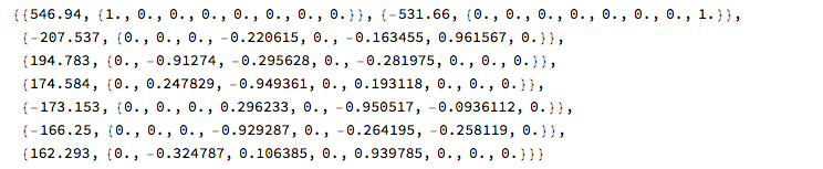
HH[base, 1, 1]
546.94
HH[base, 1, 2]
0
HH[base, 3, 5]
0.455
Spinfunctions according to mT - value
wf = Function[x, Select[base, Total[List @@ #] == 2 x &]] /@ mT

Hamilton - Submatrices
HSM[j_] := (nn = Length[wf[[j]]];
  Table[HH[wf[[j]], m, n], {m, 1, nn}, {n, 1, nn}])
HSM[2];
% // MatrixForm

HSM[2] /. {\[Nu][10] -> -\[Nu], \[Nu][11] -> 0, \[Nu][12] -> \[Nu],
   J[1, 2] -> J, J[1, 3] -> J, J[2, 3] -> J};
  % // MatrixForm

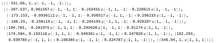
Get Eigenstates [Congruent] all sets { freq, eigenvector } for different spin-states (mT values)
frevec[n_] := Module[{es},
  es = Eigensystem[HSM[n]];
  {#[[1]], #[[2]].wf[[n]]} & /@ Transpose[es]
  ]
eigenstates = frevec /@ Range[nsp + 1]
Operator for calculating relative intensities
IOP[x_] := Sum[Ix[x, n], {n, 1, nsp}]
Calculating a spectral line = difference of eigenvalues and intensity
line[a_, b_] := Module[{},
  freq = Abs[a[[1]] - b[[1]]];
  m2 = (Expand[a[[2]] IOP[b[[2]]]] /. rscp)^2;
  {freq, Sqrt[m2]}]
Lorentzfunction
LF[x_, x0_, a_, h_] := Module[{},
  If[h == 0, h = 1];
  1/Sqrt[Pi] (a h/2)/(h^2/4 + Pi (x - x0)^2)]
Calculating the spectrum
spec = Table[0, {numberoflines}];
nL = 0;
Do[
lk = Length[eigenstates[[i]]];
lk1 = Length[eigenstates[[i + 1]]];
Do[
Do[
nL = nL + 1;
spec[[nL]] = line[eigenstates[[i, m]], eigenstates[[i + 1, n ]]],
{n, 1, lk1}
],
{m, 1, lk}
],
{i, 1, Length[eigenstates] - 1}];
normalizer = Max[Transpose[spec][[2]]];
bb = {.95 Min[Transpose[spec][[1]]], 1.05 Max[Transpose[spec][[1]]]};
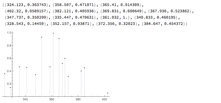
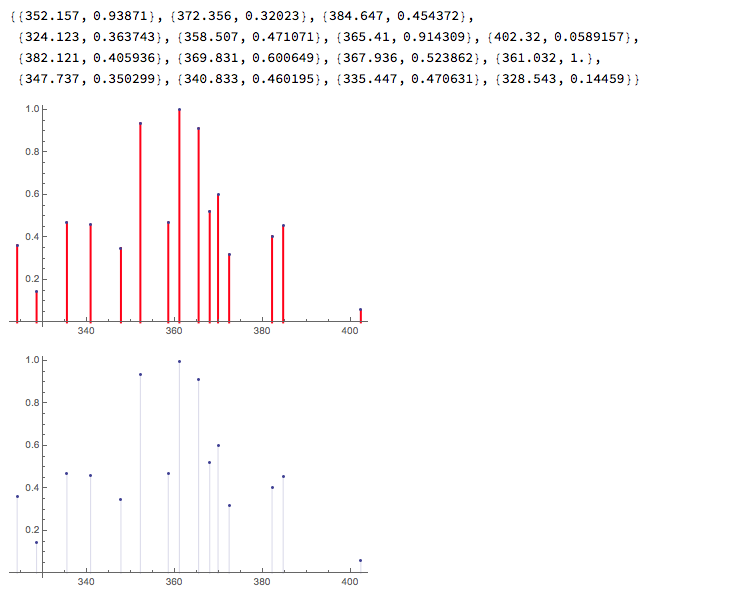
spec = {#[[1]], #[[2]]/normalizer} & /@ spec;
spec
pl1 = ListPlot[spec, Filling -> Axis]
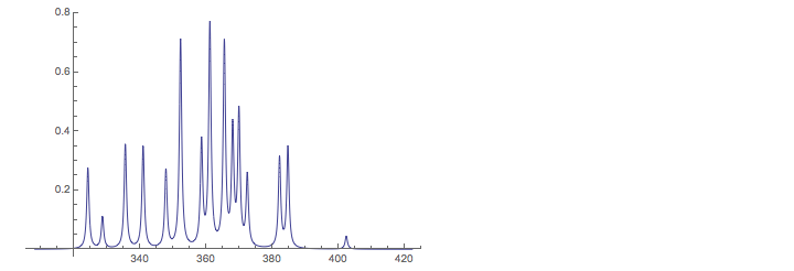
Show the spectrum with lines
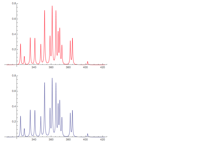
pl2 = Plot[
  Plus @@ (LF[x, #[[1]], #[[2]], 1.5] & /@ spec), {x, bb[[1]],
   bb[[2]]}, PlotRange -> All, AxesOrigin -> {320, 0}]
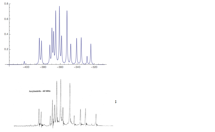
For some physical reason spectra are recorded so that frequencies grow from right to left. So the plot is reversed and compared to the experimental spectrum ( see http://www.users.csbsju.edu/~frioux/nmr/Speclab4.htm ) which is given below the plot.
pl3 = Plot[
  Plus @@ (LF[-x, #[[1]], #[[2]], 1.5] & /@ spec), {x, -bb[[2]], -bb[[
     1]]}, PlotRange -> All]
Part 2
nsp = 3;
Input of Parameters
freqs = {372.2, 364.4, 342, 6.083, 5.8};
JJ = ( {
    {0, .91, 17.9, 1, 1, 1},
    {0, 0, 11.75, 1, 1, 1},
    {0, 0, 0, 1, 1, 1},
    {0, 0, 0, 0, 1, 1},
    {0, 0, 0, 0, 0, 1},
    {0, 0, 0, 0, 0, 0}
   } );
Do[\[Nu][i] = freqs[[i]], {i, 1, nsp}];
Do[J[i, k] = JJ[[i, k]], {i, 1, nsp - 1}, {k, i + 1, nsp}];
number of lines to be expected and dimension ot (total) spin - space (at least for spin 1/2 )
numberoflines = Binomial[2 nsp, nsp - 1]
dimspsp = 2^nsp
15
8
spin operators for spin I = 1/2
ix = ( { {0, 1}, {1, 0} } )/2;
iy = ( { {0, -I}, {I, 0} } )/2;
iz = ( {{1, 0}, {0, -1} } )/2;
this function constructs the spin operator of particle j as matrix in the spin space of n particles
Op[op_, n_, j_] := Module[{x, m},
  x = Join[Table[{{1, 0}, {0, 1}}, {j - 1}], {op},
    Table[{{1, 0}, {0, 1}}, {n - j}]];
  m = SparseArray[KroneckerProduct[Sequence @@ x]]
  ]
oIx[j_] := Op[ix, nsp, j]
oIy[j_] := Op[iy, nsp, j]
oIz[j_] := Op[iz, nsp, j]
Hamiltonian
HH = \!\(
\*UnderoverscriptBox[\(\[Sum]\), \(i = 1\), \(nsp\)]\(\[Nu][i] oIz[
     i]\)\) + \!\(
\*UnderoverscriptBox[\(\[Sum]\), \(i = 1\), \(nsp - 1\)]\(
\*UnderoverscriptBox[\(\[Sum]\), \(j = i + 1\), \(nsp\)]J[i,
      j] \((oIx[i] . oIx[j] + oIy[i] . oIy[j] + oIz[i] . oIz[j])\)\)\)
SparseArray[SequenceForm["<", 32, ">"], {8, 8}]
Eigensystem for the Hamilton - Operator
est = Transpose[Eigensystem[HH]]
Intensity operator
IOP1 = \!\(
\*UnderoverscriptBox[\(\[Sum]\), \(j = 1\), \(nsp\)]\(oIx[j]\)\)
SparseArray[SequenceForm["<", 24, ">"], {8, 8}]
line1[a_, b_] := Module[{},
  freq = Abs[a[[1]] - b[[1]]];
  m2 = (a[[2]].IOP1.b[[2]])^2;
  {freq, Sqrt[m2]}]
Calculate spectrum, show it and display result from part 1
spec1 = Table[0, {Binomial[dimspsp, 2]}];
nL = 0;
Do[
 Do[
  nL = nL + 1;
  spec1[[nL]] = line1[est[[u]], est[[v]]],
  {u, v + 1, dimspsp}
  ],
 {v, 1, dimspsp - 1}
 ]
spec1 = Select[spec1, #[[2]] > 0. &];
normalizer = Max[Transpose[spec1][[2]]];
bb = {.95 Min[Transpose[spec][[1]]], 1.05 Max[Transpose[spec][[1]]]};
spec1 = {#[[1]], #[[2]]/normalizer} & /@ spec1;
spec1
ListPlot[spec1, Filling -> Axis, FillingStyle -> Directive[Red, Thick]]
Show[pl1]
Plot the spectrum and compare with the result of the 1 st part
pl4 = Plot[
  Plus @@ (LF[x, #[[1]], #[[2]], 1.5] & /@ spec1), {x, bb[[1]],
   bb[[2]]}, PlotRange -> All, PlotStyle -> Red]
Show[pl2]
 Attachments:


