The notion of particles filters
The idea I would like to share today is borrowed from a quiz question from Udacity's "Introduction to Computer Vision" course. Although the question is a simple one, the notion built around it highlights the importance of "particle filters". Particle filters - like Kalman filter - is a filtering technique that is utilized to better localize a signal using a prediction (from a model) and measured observation. However, in contrast to the Kalman filter, the solution is not acquired analytically/numerically but via the use of discrete particles. The signal can be N-Dimensional and the number of particles scale accordingly.
One use of particle filters can be to track objects. The usage of particles will assume a knowledge of a prior distribution (created from a model or hypothesis). The prediction is basically a vague but reasonable attempt to localize the object. A given number of particles are created and sampled from the prior distribution. Thereafter, a measured observation - a measure of how likely it is to get the measurement value given the object is at that point - is used to re-weight the particles. The time is advanced, particles displaced and the cycle continues.
Now about the puzzled ant
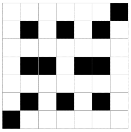
The question deals with an ant roaming on a rectangular grid of cell coloured either black or white. The ant knows the map, however, has lost track of its current location. We can create a very simple particle filter for such a case to narrow down the possible locations where the ant might be. The only information the ant has is an account of the directions it has turned so far and the colour observed along the way.
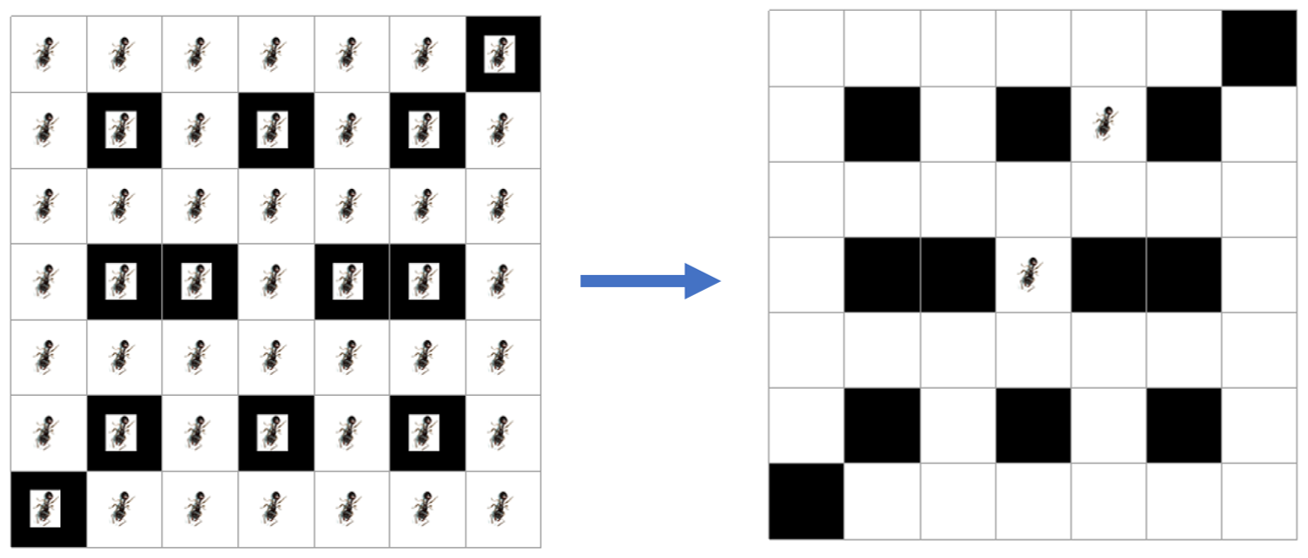
The iterative scheme - implemented using particle filters - to solve the problem is a simple one: 1. we start by assuming that the ant is everywhere, its location being tracked by individual particles distributed ubiquitously in the grid. 2. the ants motion displaces the particles along the direction of motion. 3. the particles which move outside the map or those that do not correspond to the observed colour after each motion step are discarded.
Information at hand
Below is the map over which the ant moves

Our ant being a computer science ant (as the authors state) can only moves up, down, right and left. The information the ant has about its motion is as follow:
moved "up" observed white tile
moved "left" observed black tile
moved "up" twice and each time observed a white tile
moved "right" observed a black tile
currently on a white tile
The code to solve the problem was implemented as follows:
antimage = Import["https://cdn.orkin.com/images/ants/pavement-ant-illustration_1936x1600.jpg"]
matrix = Table[{i, j}, {i, 7}, {j, 7}];
indices = Flatten[matrix, 1];
matrix[[All, All]] = "Ant";
blackpos = {{1, 7}, ## & @@ Thread[{2, Range[2, 6, 2]}], {4, 2}, {4, 3}, {4, 5}, {4, 6},
## & @@ Thread[{6, Range[2, 6, 2]}], {7, 1}};
whitepos = Complement[indices, blackpos];
s = SparseArray[Join[Thread[whitepos -> 1], Thread[blackpos -> 0]]];

Clear@func;
func[grid_, {obs_, move_}] := Module[{tempg, posAntOld, posAntNew},
  If[obs == 1, tempg = ReplacePart[grid, blackpos -> 0],
   tempg = ReplacePart[grid, whitepos -> 0]];
  posAntOld = Position[tempg, "Ant"];
  Switch[move, "up", tempg = Join[Rest@tempg, {ConstantArray[0, 7]}],
   "left",
   tempg = Insert[tempg[[All, 2 ;;]] // Transpose,
      ConstantArray[0, 7], -1] // Transpose,
   "right",
   Insert[tempg[[All, ;; -2]] // Transpose, ConstantArray[0, 7], 1] //
     Transpose,
   "down", tempg = Prepend[Most@tempg, {ConstantArray[0, 7]}],
   Null, tempg]
]
the function is called iteratively
sol = FoldList[func, matrix, Thread[{{1, 0, 1, 1, 0, 1}, {"up", "left", "up", "up", "right", Null}}]];
list = Map[Inset[antimage, # - 0.75, # + 0.75, 0.5] & /@ Position[#, "Ant"] &, sol];
seq = Rotate[ArrayPlot[Transpose@s, ColorRules -> {1 -> White, 0 -> Black}, Mesh -> All, Epilog -> #,
DataReversed -> {True, False}], -Pi/2] & /@ list;

GraphicsRow[seq, ImageSize -> Full]
the evolution of the system can be seen below: 
A zoomed in version of the initial and final state:

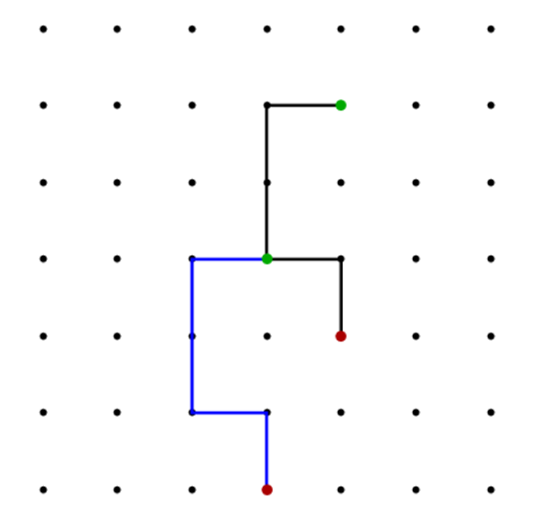
As is evident from the last grid on the right, we are left with just two possible tiles of which one is where the ant can possibly be. Both locations are equally valid. We can find out the paths that the ant could take from the start to reach either destinations.
backtrackRule = {"up" -> "down", "left" -> "right", "right" -> "left", "down" -> "up"};
backtrackValRule = Dispatch[{"down" -> {1, 0}, "up" -> {-1, 0}, "right" -> {0, 1}, "left" -> {0, -1}}];
backtrackpos = Reverse@{"up", "left", "up", "up", "right"} /. backtrackRule /. backtrackValRule;

backtracksol = FoldList[#1 + #2 &, #, backtrackpos] & /@ {{2, 5}, {4, 4}}; (*where the two pts are the possible destinations*)

Rotate[Show[ListPlot[indices, Axes -> False, PlotStyle -> Black, AspectRatio -> 1], Graphics[{{{Thick, Line@backtracksol[[1]]},
{Blue, Thick, Line@backtracksol[[2]]}}, {Darker@Green, PointSize[Large], Point[{{2, 5}, {4, 4}}]},
{Darker@Red, PointSize[Large], Point[Last[{##}] & @@@ backtracksol]}}]], -Pi/2]
possible paths:

In near future, I aspire to implement a probabilistic approach to track multiple fluorescent particles in cells - possibly a pseudocode by Godinez et al.