Mathematical approaches become more and more relevant in policing. In the CBS series Numb3rs a mathematician genius helps his FBI agent brother to solve crime using maths. It turns out that much of the maths used in the series is actually relevant for law enforcement and indeed Wolfram Inc advised the maker of the program on the maths. There are many approaches described in the series and in the book "The numbers behind Numb3rs": geoprofiling is one of the most prominent methods.

It turns out that Los Angeles mathematicians work together with the police on a methods called predictive policing, where data and mathematical approaches are being used to direct police officers to locations with a high probability of a crime being committed. A substantial drop in crime rates has been reported. The mathematician Prof. Andrea Bertozzi is leading efforts in predictive policing. Here is a brilliant talk on one of the approaches. In the video they discuss a model based on the (near) repeat victimisation theory - which is based on the observation that often the same or similar targets have a higher likelihood of being targeted again.

In this post I will implement (something similar to) the discrete version of their model and then extend it using some data. We will obtain graphics like this one that shows how crime hotspots develop over time.

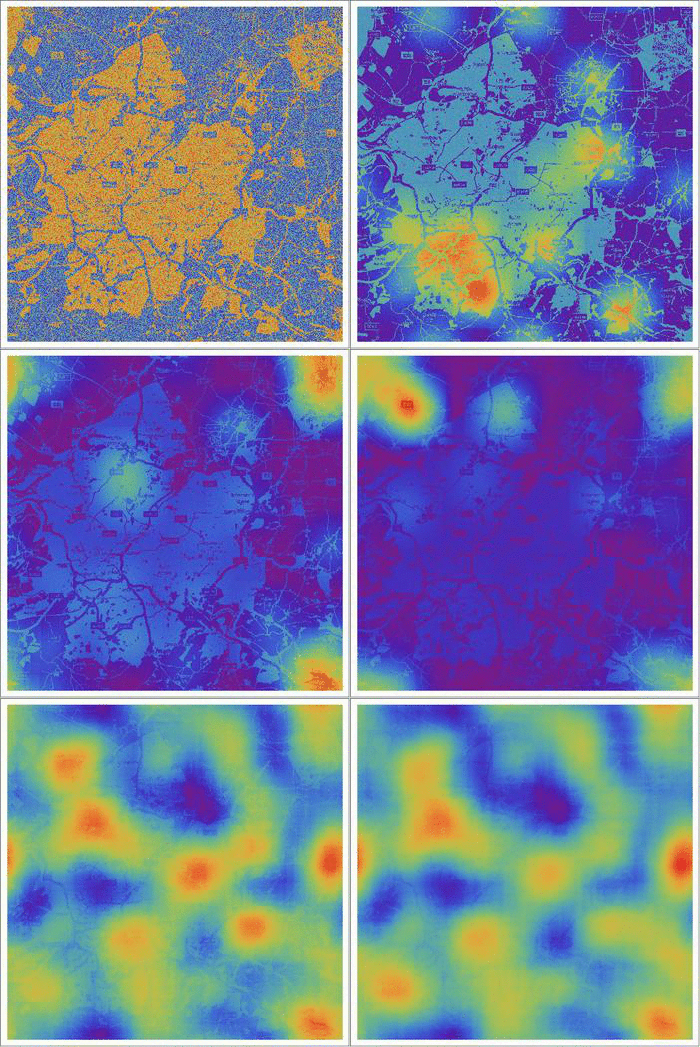
A higher resolution video can be found on Youtube.

Exploratory data analysis

We start by analysing some actual crime data made available by the police in the UK. It is freely available at the website: https://data.police.uk/data/. There is a wealth of data - and actually it is quite frightening to see how many crimes are committed. I suppose that this data would be great for the Wolfram Data Repository. I will start with the December 2016 data for Avon-and-Summerset. Once downloaded I can import the data.

data = Import["~/Desktop/Crime/2016-12/2016-12-avon-and-somerset-street.csv"];
data[[1 ;; 2]] // Transpose // TableForm

I only show one dataset. There are 13751 entries in this particular file. We can now look at the tally of the different crime types:

Reverse@SortBy[Tally[data[[2 ;;, 10]]], Last] // TableForm

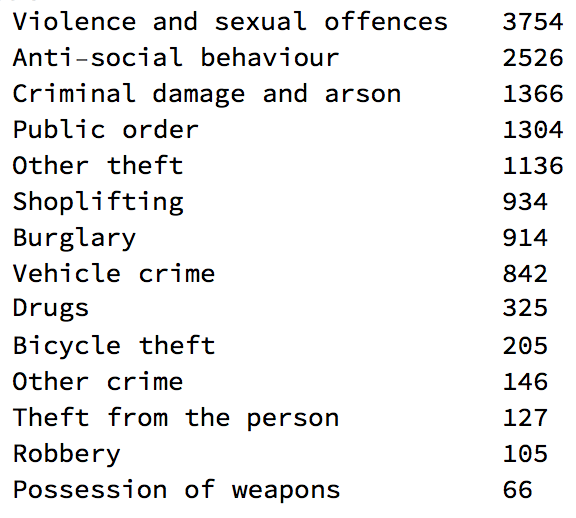
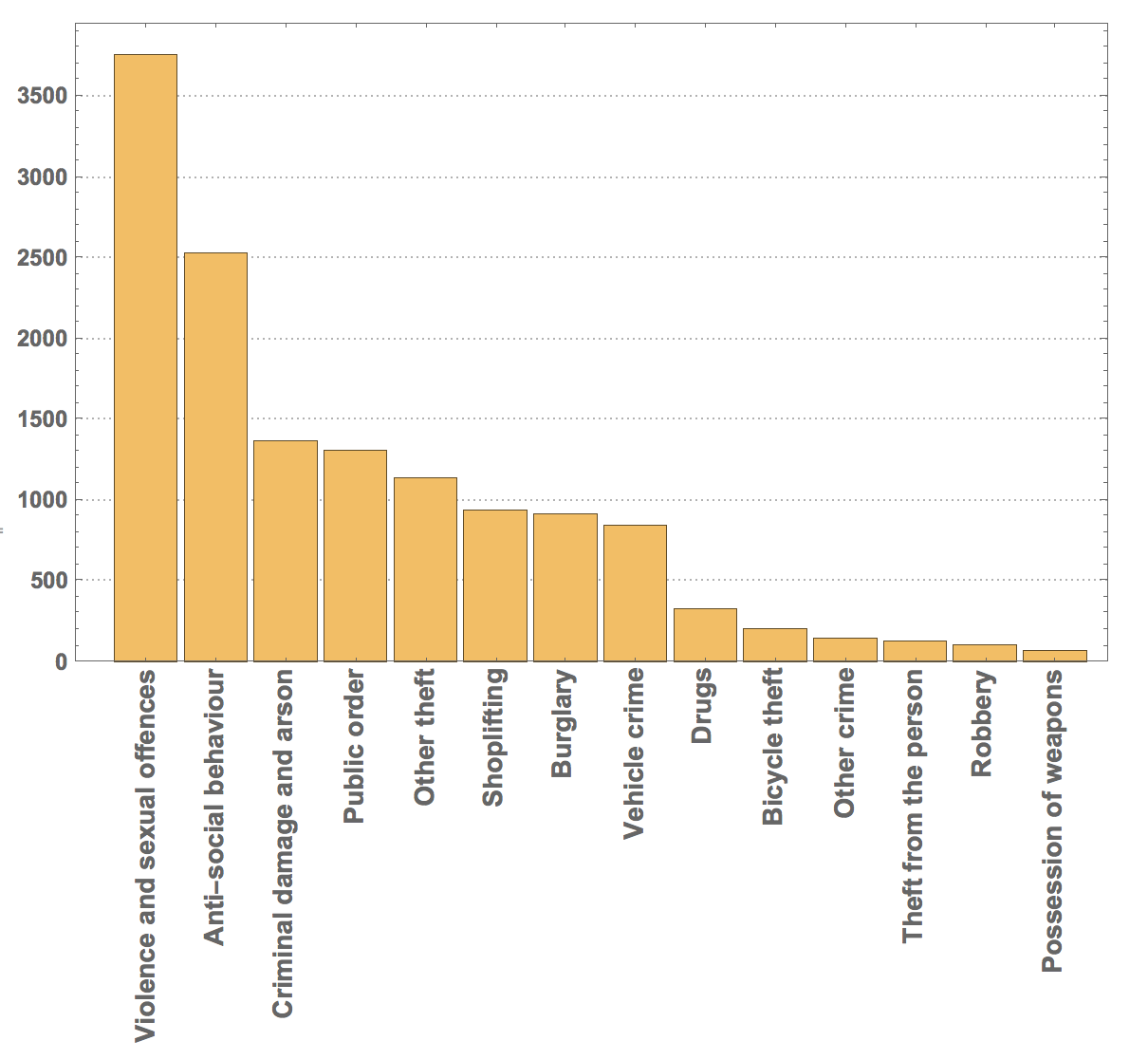
So violence and sexual offences "top" the list. The following bar chart visualises the this tally:

BarChart[(Reverse@SortBy[Tally[data[[2 ;;, 10]]], Last])[[All, 2]], 
ChartLabels -> (Rotate[Style[#[[1]], 14], Pi/2.] & /@ (Reverse@SortBy[Tally[data[[2 ;;, 10]]], Last])), LabelStyle -> Directive[Bold, Medium], ImageSize -> Large, PlotTheme -> "Detailed"]

Next we define rules to label the different types of crime:

assignments = Table[(Sort[Tally[data[[2 ;;, 10]]]])[[k, 1]] -> k, {k, 1, Length[Tally[data[[2 ;;, 10]]]]}]

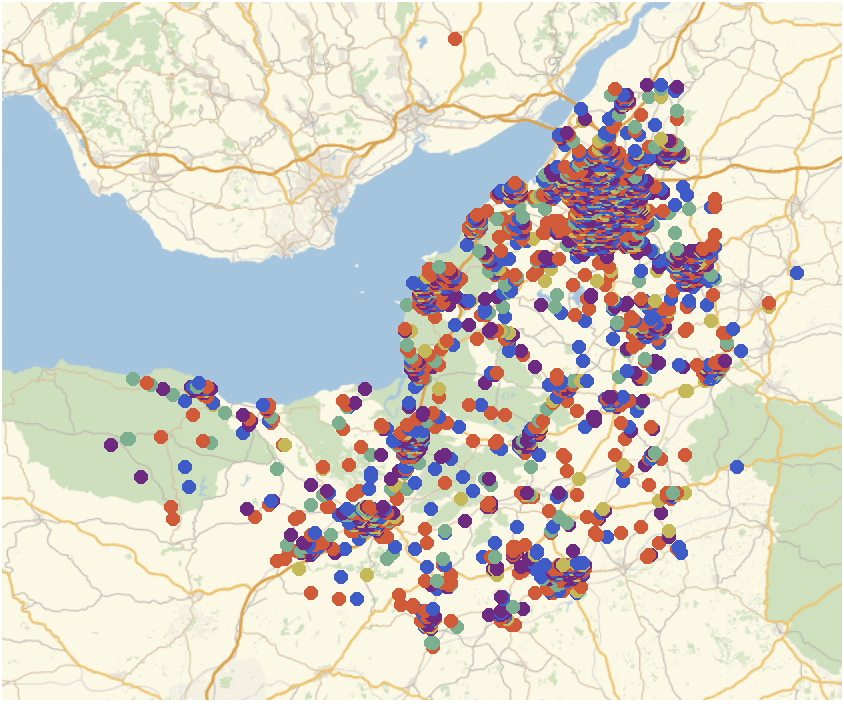
We can then generate a list of locations and types of crime and plot it:

crimelocandtype = 
  Select[(data[[2 ;;, {5, 6, 10}]] /. assignments ), StringQ[#[[1]]] == False &];
GeoRegionValuePlot[GeoPosition[Reverse[{#[[1]], #[[2]]}]] -> #[[3]]/Length[assignments] & /@ crimelocandtype, 
ColorFunction -> "Rainbow", GeoRange -> {{50.7608, 51.748}, {-3.92098, -2.0238}}]

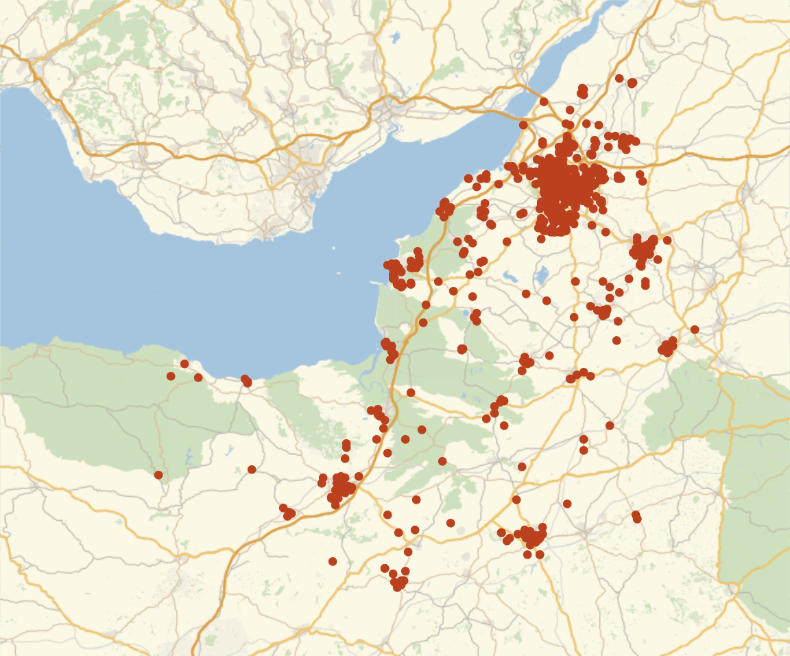
We can also look at particular types of crime and plot that:

burglaries = Select[crimelocandtype, #[[-1]] == 3 &];
posBurglaries = 
 GeoListPlot[GeoPosition[Reverse[{#[[1]], #[[2]]}]] & /@ burglaries, 
  GeoRange -> {{50.7608, 51.748}, {-3.92098, -2.0238}}, 
  ImageSize -> Large]

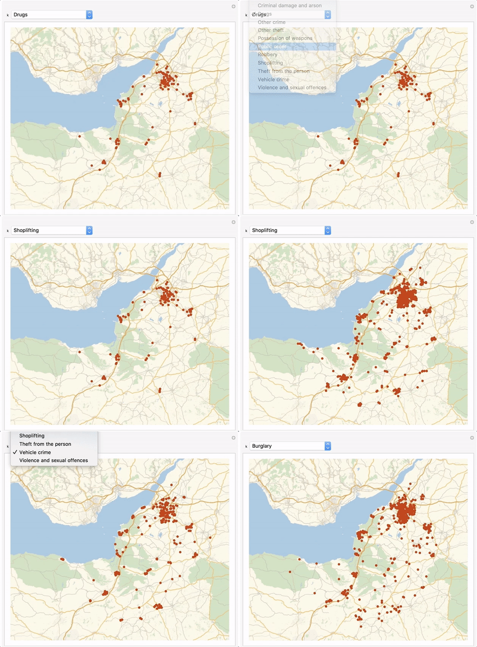
We can wrap that into an interactive Manipulate environment:

Manipulate[
 GeoListPlot[
  GeoPosition[Reverse[{#[[1]], #[[2]]}]] & /@ 
   Select[crimelocandtype, #[[-1]] == 
      assignments[[Position[assignments, k][[1, 1]]]][[2]] &], 
  GeoRange -> {{50.7608, 51.748}, {-3.92098, -2.0238}}, 
  ImageSize -> Large], {k, assignments[[All, 1]]}]

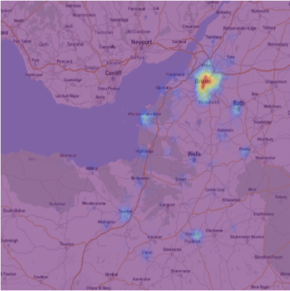
We can of course also calculate the distribution of a particular crime, here burglary.

burglaryDistribution = 
SmoothKernelDistribution[
DeleteCases[burglaries[[All, {2, 1}]], {"", ""}], "SheatherJones"];
cplot = ColorReplace[
ContourPlot[PDF[burglaryDistribution, {y, x}], 
Evaluate@
Flatten[{x, {#[[1, 1, 2]], #[[2, 1, 2]]} &@(GeoPosition /@ 
Transpose[{{50.7608, 51.748}, {-3.92098, -2.0238}}])}], 
Evaluate@
Flatten[{y, {#[[1, 1, 1]], #[[2, 1, 1]]} &@(GeoPosition /@ 
Transpose[{{50.7608, 51.748}, {-3.92098, -2.0238}}])}], 
ColorFunction -> "Rainbow", Frame -> False, PlotRange -> All, 
Contours -> 405, MaxRecursion -> 2, 
ColorFunction -> ColorData["TemperatureMap"], 
PlotRangePadding -> 0, ContourStyle -> None, ImageSize -> Full], 
White -> RGBColor[
0.4691184586237173, 0.10979455248315054`, 0.5269517756641199]];
ImageCompose[
ImageResize[
Image[GeoGraphics[
Entity["City", {"Bristol", "Bristol", "UnitedKingdom"}], 
GeoRange -> {{50.7608, 51.748}, {-3.92098, -2.0238}}]], 
ImageDimensions@Image[cplot]], {Image[cplot], 0.6}]

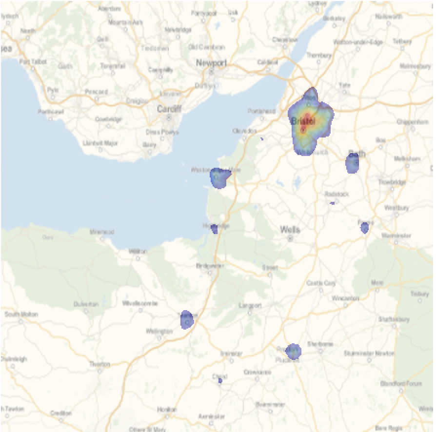
Alternatively, we can remove very low incident rates.

cplot2 = ColorReplace[
   ContourPlot[PDF[burglaryDistribution, {y, x}], 
    Evaluate@
     Flatten[{x, {#[[1, 1, 2]], #[[2, 1, 2]]} &@(GeoPosition /@ 
          Transpose[{{50.7608, 51.748}, {-3.92098, -2.0238}}])}], 
    Evaluate@
     Flatten[{y, {#[[1, 1, 1]], #[[2, 1, 1]]} &@(GeoPosition /@ 
          Transpose[{{50.7608, 51.748}, {-3.92098, -2.0238}}])}], 
    ColorFunction -> "Rainbow", Frame -> False, PlotRange -> All, 
    Contours -> 405, MaxRecursion -> 2, 
    ColorFunction -> ColorData["TemperatureMap"], 
    PlotRangePadding -> 0, ContourStyle -> None, ImageSize -> Full], 
   RGBColor[
    0.4691184586237173, 0.10979455248315054`, 0.5269517756641199] -> 
    White];
ImageCompose[
 ImageResize[
  Image[GeoGraphics[
    Entity["City", {"Bristol", "Bristol", "UnitedKingdom"}], 
    GeoRange -> {{50.7608, 51.748}, {-3.92098, -2.0238}}]], 
  ImageDimensions@Image[cplot2]], {Image[cplot2], 0.5}]

We can also focus on the city of Bristol.

burglaryDistribution = 
  SmoothKernelDistribution[
   Select[DeleteCases[burglaries[[All, {2, 1}]], {"", ""}], 
    51.32107 < #[[1]] < 51.58066 && -2.70098 < #[[2]] < -2.396148 &] ,
    "SheatherJones"];
cplot3 = ColorReplace[
   ContourPlot[PDF[burglaryDistribution, {y, x}], 
    Evaluate@
     Flatten[{x, {#[[1, 1, 2]], #[[2, 1, 2]]} &@(GeoPosition /@ 
          Transpose[{{51.58066, 51.32107}, {-2.70098, -2.396148}}])}],
     Evaluate@
     Flatten[{y, {#[[1, 1, 1]], #[[2, 1, 1]]} &@(GeoPosition /@ 
          Transpose[{{51.58066, 51.32107}, {-2.70098, -2.396148}}])}],
     ColorFunction -> "Rainbow", Frame -> False, PlotRange -> All, 
    Contours -> 405, MaxRecursion -> 2, 
    ColorFunction -> ColorData["TemperatureMap"], 
    PlotRangePadding -> 0, ContourStyle -> None, ImageSize -> Full], 
   RGBColor[
    0.4691184586237173, 0.10979455248315054`, 0.5269517756641199] -> 
    White];
ImageCompose[
 ImageResize[
  Image[GeoGraphics[
    Entity["City", {"Bristol", "Bristol", "UnitedKingdom"}], 
    GeoRange -> {{51.58066, 51.32107}, {-2.70098, -2.396148}}, 
    ImageSize -> Full]], 
  ImageDimensions@Image[cplot]], {Image[cplot3], 0.65}]

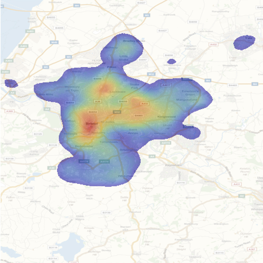
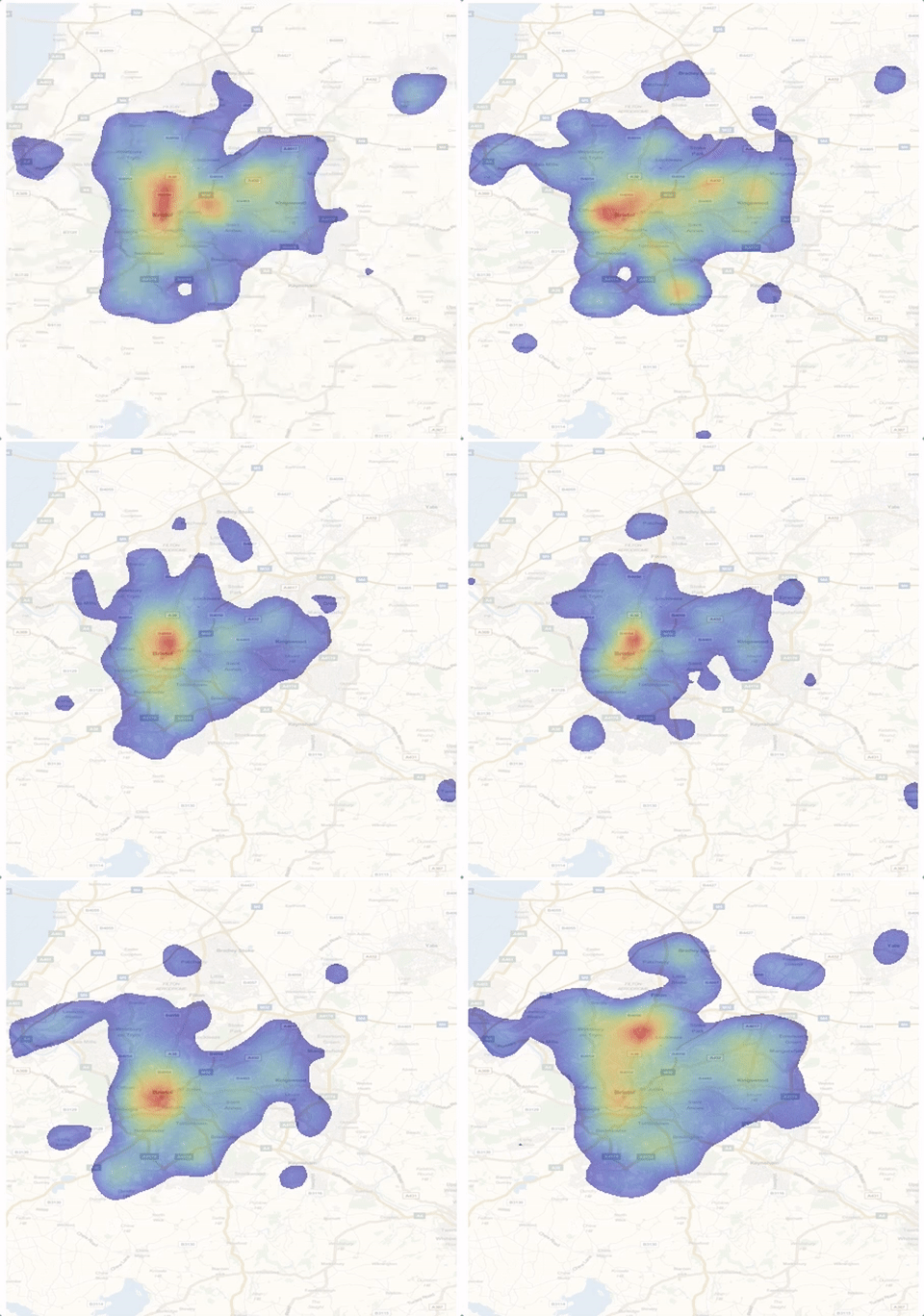
Next, we can investigate how this distribution changes over time. We will need more data and, as it turns out there are more categories of crime in the entire dataset.

assignments = 
  Table[Sort[Tally[data[[2 ;;, 10]]]][[k, 1]] -> k, {k, 1, 
    Length[Tally[data[[2 ;;, 10]]]]}];
filenames = FileNames["*", "~/Desktop/Crime/*"];
frames = {};
Monitor[Do[data = Import[filenames[[k]]];
   crimelocandtype = 
    Select[(data[[2 ;;, {5, 6, 10}]] /. assignments ), 
     StringQ[#[[1]]] == False &];
   burglaries = Select[crimelocandtype, #[[-1]] == 3 &];
   burglaryDistribution = 
    SmoothKernelDistribution[
     Select[DeleteCases[burglaries[[All, {2, 1}]], {"", ""}], 
      51.32107 < #[[1]] < 
         51.58066 && -2.70098 < #[[2]] < -2.396148 &] , 
     "SheatherJones"];
   cplot3 = 
    ColorReplace[
     ContourPlot[PDF[burglaryDistribution, {y, x}], 
      Evaluate@
       Flatten[{x, {#[[1, 1, 2]], #[[2, 1, 2]]} &@(GeoPosition /@ 
            Transpose[{{51.58066, 
               51.32107}, {-2.70098, -2.396148}}])}], 
      Evaluate@
       Flatten[{y, {#[[1, 1, 1]], #[[2, 1, 1]]} &@(GeoPosition /@ 
            Transpose[{{51.58066, 
               51.32107}, {-2.70098, -2.396148}}])}], 
      ColorFunction -> "Rainbow", Frame -> False, PlotRange -> All, 
      Contours -> 405, MaxRecursion -> 2, 
      ColorFunction -> ColorData["TemperatureMap"], 
      PlotRangePadding -> 0, ContourStyle -> None, ImageSize -> Full],
      RGBColor[
      0.4691184586237173, 0.10979455248315054`, 0.5269517756641199] ->
       White];
   AppendTo[frames, 
    ImageCompose[
     ImageResize[
      Image[GeoGraphics[
        Entity["City", {"Bristol", "Bristol", "UnitedKingdom"}], 
        GeoRange -> {{51.58066, 51.32107}, {-2.70098, -2.396148}}, 
        ImageSize -> Full]], 
      ImageDimensions@Image[cplot]], {Image[cplot3], 0.65}]], {k, 1, 
    Length[filenames]}];, k]
Monitor[Do[
  Export["~/Desktop/Bristolhotspotmovie/frameHR" <> 
    ToString[1000 + k] <> ".jpg", frames[[k]]], {k, 1, 
   Length[frames]}], k]

We can play this with

ListAnimate[frames]

Modelling repeat victimisation

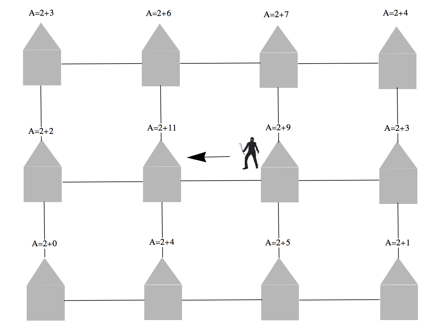
We will build a model which is very similar to the model of Prof Bertozzi. We start out with a grid of houses. Each has a base attractivity for burglars and "added attractivity" according to the history of close burglarlies. Burglars are placed randomly on the grid and tend to move towards houses with higher attractivity.

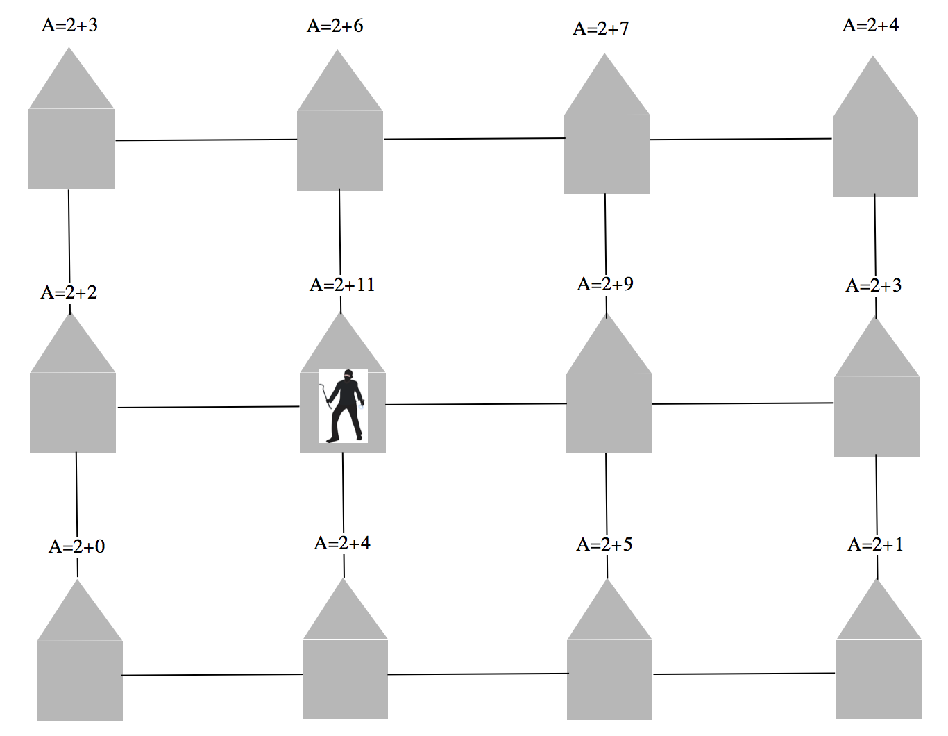
With a certain probably proportional to the attractiveness the burglar decides to raid the house.

That changes the "added attractivity" of the house that was attacked and of the neighbouring house. This added attractivity decays over time. When a burglar strikes he is removed from the grid and replaced by a new burglar, which is added at a random position.

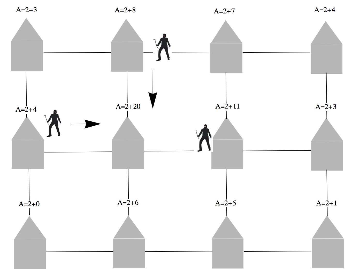
The process is then iterated.

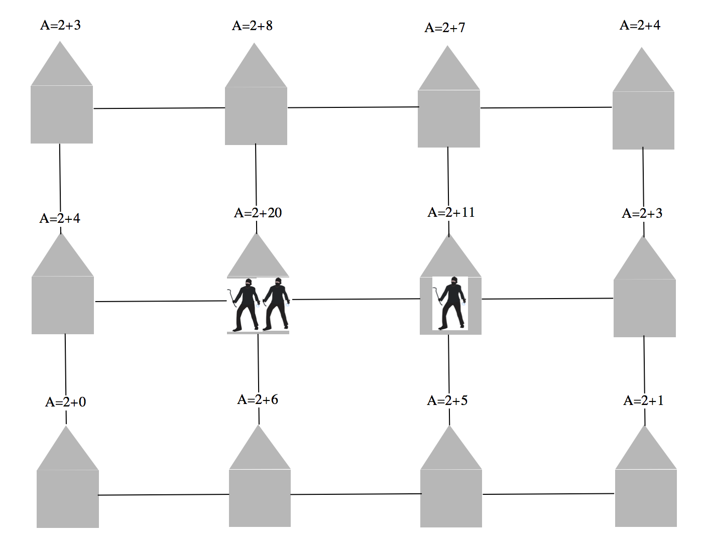
The number of burglars is kept constant.

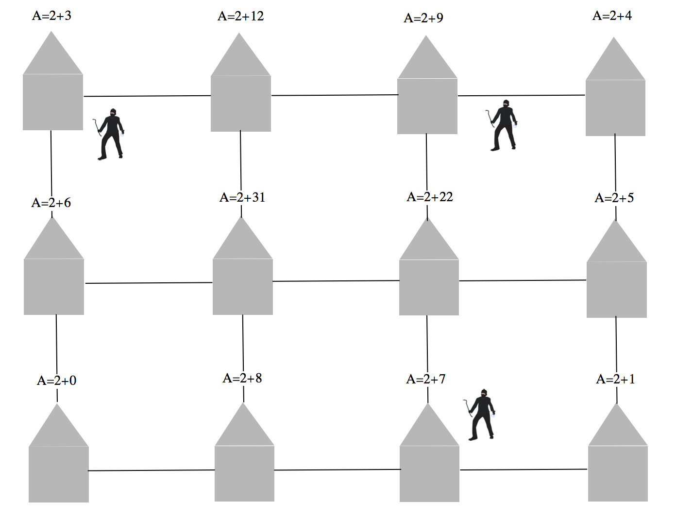
We also introduce a "sure-hit-attractivity", i.e. if a house reaches that limit and a burglar gets there, they will definitely strike. Here is the implementation of that process.

ClearAll["Global`*"](*MS*)
(*Initialisation*)
M = 200; Mrobbers = \
200; surehitattractiveness = 20.; addedattractiveness = 10.;
decay = 0.1;(*decay=0.01*)
b = 10; b = 20;(*b=5*)
(*Good:
M=200;Mrobbers=200;surehitattractiveness=20.;addedattractiveness=10;
decay=0.1; b=20; *)
basematrix = ConstantArray[2., {M, M}];
randomattractiveness = RandomReal[10., {M, M}];(*10*)

attractiveness = basematrix + randomattractiveness;
placerobbers = RandomInteger[{1, M}, {Mrobbers, 2}];
output = {};

Monitor[Do[
  (*Update robber position *)

  neighbours = 
   Table[placerobbers[[k]] - # /. {0 -> M, M + 1 -> 1} & /@ {{-1, 
       0}, {1, 0}, {0, -1}, {0, 1}}, {k, 1, Length[placerobbers]}];
  moves = 
   Table[{attractiveness[[#[[1]], #[[2]]]], #} & /@ 
     neighbours[[k]], {k, 1, Length[placerobbers]}];
  placerobbers = RandomChoice[Rule @@ Transpose[#]] & /@ moves;
  (*Update attractiveness*)

  change = ConstantArray[
    0., {M, M}]; (change[[#[[1, 1]], #[[1, 2]]]] = 
      change[[#[[1, 1]], #[[1, 2]]]] + #[[2]]) & /@ ({#, 
       RandomChoice[{Min[
           attractiveness[[#]]/(surehitattractiveness + 10^(-7)), 
           1], (1. - 
            Min[attractiveness[[#]]/(surehitattractiveness + 10^(-7)),
              1])} -> {addedattractiveness, 0}]} & /@ placerobbers);

  change2 = ListConvolve[GaussianMatrix[b], change, M - b];
  change = 
   Max[Flatten[change]]/(Max[Flatten[change2]] + 10^(-7))*change2;
  randomattractiveness = (1. - decay) (randomattractiveness + change);
   attractiveness = basematrix + randomattractiveness;
  (*Remove and add robbers*)

  placerobbers = 
   DeleteCases[placerobbers, Position[change, n_ /; n > 9]];
  While[Length[placerobbers] < Mrobbers, 
   AppendTo[placerobbers, RandomInteger[{1, M}, 2]]];
  AppendTo[output, ArrayPlot[attractiveness, ColorFunction -> "Rainbow", PlotRange -> 80]];, {l, 1000}], l]

Note that there are several "tricks" that make the code run faster. The most obvious is that I do not add the "addedatractiveness" to all the neighbours one by one, but use the function ListConvolve with the GaussianMatrix.

Here are some snapshots from the model.

Grid[Partition[output[[1 ;; ;; 83]], 4]]

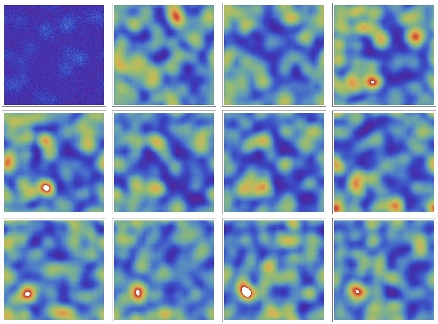
Hotspots of crime seem to develop spontaneously and move. So we have moving hotspots - this is interesting because the underlying base attractivity is uniform. This means that we have a sort of self-organising pattern of hot spots. This, of course, depends on the parameters we choose. The following choice for the initialisation leads to no patters at all.

(*Initialisation*)
M = 200; Mrobbers = 200; surehitattractiveness = \
20.; addedattractiveness = 10; addedattractiveness = 3;
decay = 0.1; decay = 0.002;(*decay=0.01*)
b = 10; b = 20; b = 2;(*b=5*)

This last set of parameters will lead to stable/periodic spots, i.e. spots that move little over time and lie on lines.

(*Initialisation*)
M = 200; Mrobbers = 200; surehitattractiveness = \
30.; addedattractiveness = 17.;
decay = 0.03;(*decay=0.01*)
b = 10; b = 15;(*b=5*)
(*Good:
M=200;Mrobbers=200;surehitattractiveness=20.;addedattractiveness=10;
decay=0.1; b=20; *)

Here is a movie of the three situations (where the list of frames were named intuitively).

Manipulate[GraphicsRow[{framesNS[[k]], framesMS[[k]], framesSS[[k]]}, ImageSize -> 800], {k, 1, 100, 1}]

In fact, I exported the frames and used an external program to generate the animated gif.

Monitor[Do[Export["~/Desktop/SimpleBurglaryMov/tripleframesLR" <> ToString[1000 + k] <> ".jpg", 
GraphicsRow[{framesNS[[k]], framesMS[[k]], framesSS[[k]]}, ImageSize -> 600]], {k, 1, 100}], k]

Giving spatial structure to the model

We will now try to add spatial information to the model and thereby try to make it "more similar" to the data. We will use a map of Bristol as background.

backgroundmap = 
 Binarize[ColorReplace[
   GeoGraphics[
    Entity["City", {"Bristol", "Bristol", "UnitedKingdom"}], 
    GeoRange -> {{51.58066, 51.32107}, {-2.70098, -2.396148}}, 
    ImageSize -> Full], 
   RGBColor[0.7645654097466869, 0.7601412050621937, 0.7438859309145965] -> Black], 0.5]

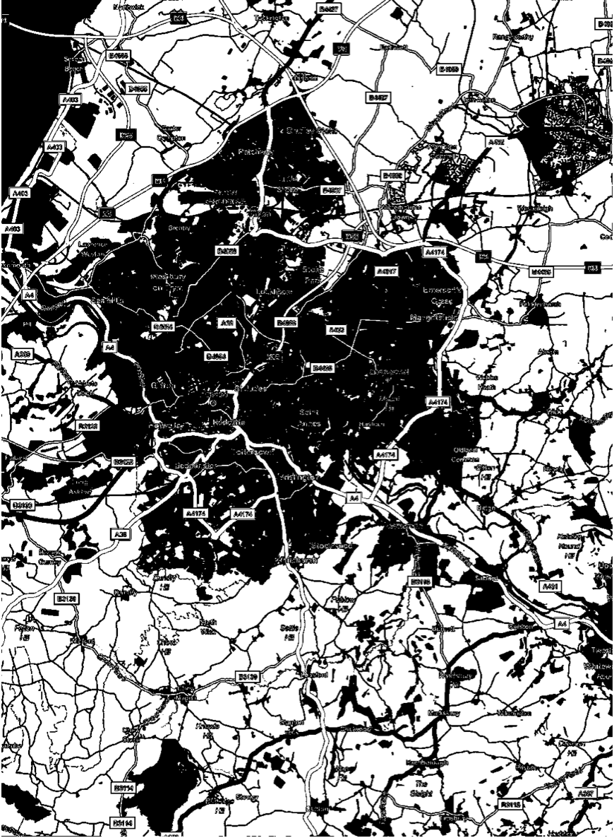
We will then crop the image. I have used the crop tool for that and attach the image so that you can work with the same file as me.

backgroundmapcropped=Import["~/Desktop/backgroundmapcropped.png"]

and determine the ImageDimensions

ImageDimensions[backgroundmapcropped]

This is 560 by 560.

Last but not least we adapt our program as to use a 560 by 560 grid and use the background map as base attractiveness. Note that we are using periodic boundary conditions.

ClearAll["Global`*"]
(*Initialisation*)
M = 560; Mrobbers = 560; surehitattractiveness = \
20.; addedattractiveness = 23.;
decay = 0.05;(*decay=0.01*)
b = 10; b = 65;(*b=5*)
(*Good:
M=200;Mrobbers=200;surehitattractiveness=20.;addedattractiveness=10;
decay=0.1; b=20; *)
basematrix = 
 ConstantArray[11., {M, M}]*(1 - ImageData[backgroundmapcropped]);
randomattractiveness = RandomReal[12, {M, M}];
attractiveness = basematrix + randomattractiveness;
placerobbers = RandomInteger[{1, M}, {Mrobbers, 2}];
output = {};

Monitor[Do[
  (*Update robber position *)

  neighbours = 
   Table[placerobbers[[k]] - # /. {0 -> M, M + 1 -> 1} & /@ {{-1, 
       0}, {1, 0}, {0, -1}, {0, 1}}, {k, 1, Length[placerobbers]}];
  moves = 
   Table[{attractiveness[[#[[1]], #[[2]]]], #} & /@ 
     neighbours[[k]], {k, 1, Length[placerobbers]}];
  placerobbers = RandomChoice[Rule @@ Transpose[#]] & /@ moves;
  (*Update attractiveness*)

  change = 
   ConstantArray[
    0., {M, M}]; (change[[#[[1, 1]], #[[1, 2]]]] = change[[#[[1, 1]], #[[1, 2]]]] + #[[2]]) & /@ 
  ({#, RandomChoice[{Min[attractiveness[[#]]/(surehitattractiveness + 10^(-7)), 1], (1. - Min[attractiveness[[#]]/(surehitattractiveness + 10^(-7)),1])} -> {addedattractiveness, 0}]} & /@ placerobbers);

  change2 = ListConvolve[GaussianMatrix[b], change, M - b];
  change = 
   Max[Flatten[change]]/(Max[Flatten[change2]] + 10^(-7))*change2;
  randomattractiveness = (1. - decay) (randomattractiveness + change);
   attractiveness = basematrix + randomattractiveness;
  (*Remove and add robbers*)

  placerobbers = DeleteCases[placerobbers, Position[change, n_ /; n > 9]];
  While[Length[placerobbers] < Mrobbers, 
  AppendTo[placerobbers, RandomInteger[{1, M}, 2]]];
  AppendTo[output, ArrayPlot[attractiveness, ColorFunction -> "Rainbow"(*,PlotRange\[Rule]30*), ImageSize -> Large]];,{l, 100}], l]

The full movie in low resolution is shown at the beginning of this post. A higher resolution video can be found on Youtube.

What next?

There are obviously many bits that can be improved. On thing that is interesting is to study the movement of the potential robbers.

ClearAll["Global`*"](*MS*)
(*Initialisation*)
M = 200; Mrobbers = \
200; surehitattractiveness = 20.; addedattractiveness = 10.;
decay = 0.1;(*decay=0.01*)
b = 10; b = 20;(*b=5*)
(*Good:
M=200;Mrobbers=200;surehitattractiveness=20.;addedattractiveness=10;
decay=0.1; b=20; *)
basematrix = ConstantArray[2., {M, M}];
randomattractiveness = RandomReal[10., {M, M}];(*10*)
attractiveness =
  basematrix + randomattractiveness;
placerobbers = RandomInteger[{1, M}, {Mrobbers, 2}];
output = {};

Monitor[Do[
  (*Update robber position *)

  neighbours = 
   Table[placerobbers[[k]] - # /. {0 -> M, M + 1 -> 1} & /@ {{-1, 
       0}, {1, 0}, {0, -1}, {0, 1}}, {k, 1, Length[placerobbers]}];
  moves = 
   Table[{attractiveness[[#[[1]], #[[2]]]], #} & /@ 
     neighbours[[k]], {k, 1, Length[placerobbers]}];
  placerobbers = RandomChoice[Rule @@ Transpose[#]] & /@ moves;
  (*Update attractiveness*)

  change = ConstantArray[
    0., {M, M}]; (change[[#[[1, 1]], #[[1, 2]]]] = 
      change[[#[[1, 1]], #[[1, 2]]]] + #[[2]]) & /@ ({#, 
       RandomChoice[{Min[
           attractiveness[[#]]/(surehitattractiveness + 10^(-7)), 
           1], (1. - 
            Min[attractiveness[[#]]/(surehitattractiveness + 10^(-7)),
              1])} -> {addedattractiveness, 0}]} & /@ placerobbers);

  change2 = ListConvolve[GaussianMatrix[b], change, M - b];
  change = 
   Max[Flatten[change]]/(Max[Flatten[change2]] + 10^(-7))*change2;
  randomattractiveness = (1. - decay) (randomattractiveness + change);
   attractiveness = basematrix + randomattractiveness;
  (*Remove and add robbers*)

  placerobbers = 
   DeleteCases[placerobbers, Position[change, n_ /; n > 9]];
  While[Length[placerobbers] < Mrobbers, 
   AppendTo[placerobbers, RandomInteger[{1, M}, 2]]];
  AppendTo[output, 
   Show[ArrayPlot[attractiveness, ColorFunction -> "Rainbow", 
     PlotRange -> 80], Graphics[{Black, Point@placerobbers}]]];, {l, 
   1000}], l]

Here are some frames from that movie.

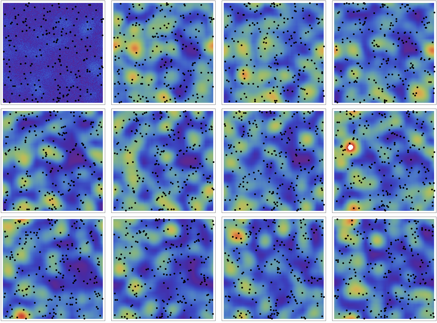
In the respective movie it is possible to follow the robbers:

Manipulate[output[[k]], {k, 1, 1000, 1}]

A high resolution video can be found of Youtube. They obviously move "randomly". Even in the model with the background attractivity they will move in a rather unconstrained way. We could obviously restrict them to the street network etc. Also, we could use data on the properties to get a better estimate of how attractive a house is. Furthermore, we could use the "heat map" data of observed crime and tweak the parameters to try and predict where robbers might strike next.

Attachments: