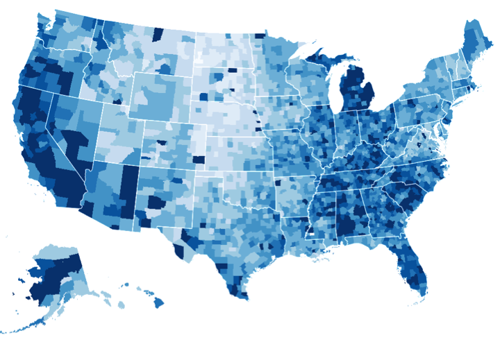
Note: I originally posted a version of this tutorial on Mathematica StackExchange. I was encouraged to make this crosspost and realized that a few things had changed since I wrote the original post. Notably, many counties now have FIPS codes. I've rewritten the text to make use of this.
Goal
The idea of the original text was to recreate Mike Bostock's D3.js choropleth map. Here is a screenshot of what it looks like: 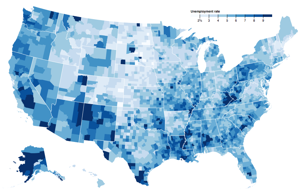
This choropleth map shows the unemployment rate in all the different US counties. I will try to use the Wolfram Knowledgebase and high-level geographics functions as much as possible. This means building my own entity store with entities that inherit properties from built-in county entities but also extend them with new properties.
Data from Wolfram Knowledgebase
GeoRegionValuePlot makes it very easy to plot data that is built into region entities. For example, this is how we can plot the fraction of each county's population that is foreign born.
counties = Cases[
   EntityList@Entity["AdministrativeDivision", {"Country" -> Entity["Country", "UnitedStates"]}],
   Entity[_, {_, _, _}] (*separates states from counties*)
   ];

GeoRegionValuePlot[counties -> "ForeignBornFraction"]
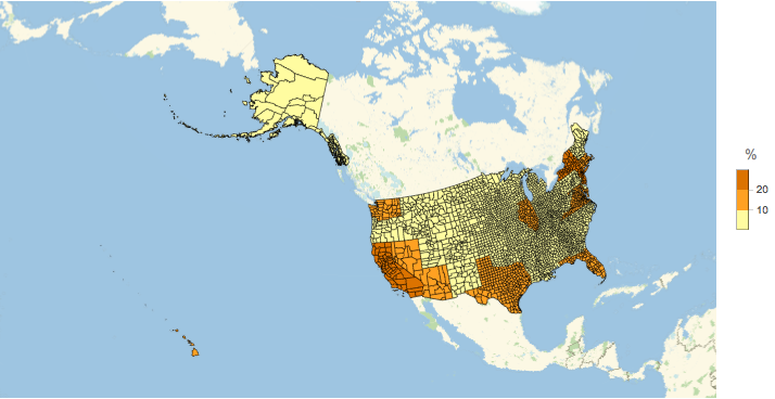
"ForeignBornFraction" is an entity property to administrative regions. Unfortunately, county properties are either missing or take the value of their state. The plot reflects the latter.
GeoRegionValuePlot is very convenient and it can be suitably styled, but Bostock's unemployment data is not available in Wolfram Knowledgebase. To be able to use the function for our purpose, we need to create our own entities where we have added Bostock's data as a property.
Custom data
We start by importing Bostock's data set.
data = <|Rule @@@ Rest@Import[
     "https://gist.githubusercontent.com/mbostock/4060606/raw/25385f68a3be5c9dbe36af27fc2498fb2aab6bc0/unemployment.tsv",
      "TSV"
      ]|>;

data // Shallow

(* Out: <|1001 -> 0.097, 1003 -> 0.091, 1005 -> 0.134, ... *)
Each entry consists of a county FIPS code and the corresponding unemployment rate. Most county entities have the FIPS code:

This makes it easy to correlate county entities with data points. However, in order to use GeoRegionValuePlot, we need entities which have the unemployment rate as one of their properties. We will achieve this by creating a new entity class, which inherits the necessary data from county entities but also includes our custom data.
getEntityIdentifier[Entity[_, {county_, state_, country___}]] := county <> "-" <> state
getEntityIdentifier[Entity[_, {"DistrictOfColumbia", _}]] := "DistrictOfColumbia"

customEntity[entity_] := If[
  ! MatchQ[entity["FIPSCode"], _Missing],
  getEntityIdentifier[entity] -> <|
    "Label" -> Style[entity["Name"], Bold],
    "ParentEntity" -> entity,
    "Unemployment" -> data[ToExpression@entity["FIPSCode"]]
    |>,
  Nothing
  ]
customEntity creates a "child entity" with the properties ParentEntity and `Unemployment. Counties which do not have a FIPS code are ignored. An example of a custom entity:

Note that we could easily add many other properties. Now create a child entity for each county:
Quiet[countyEntities = <|customEntity /@ counties|>;]
I don't know why, but it only worked if I first went to File -> Preferences -> Internet connectivity and unchecked the box "Allow the Wolfram System to access the Internet". Otherwise, the evaluation would hang forever. I put Quiet in there because otherwise it would complain about not having Internet access. Don't forget to enable the Internet connectivity again when you're done with this part, you'll need it for the geo functions.
We now create an entity store with the custom entities. This entity store comes with properties which are automatically computed from the parent entities. "Inheritance" is achieved by using the ParentEntity property to get the corresponding properties from the parent entity. The properties which are inherited have been chosen because they are the ones which are necessary to use GeoRegionValuePlot. GeoRegionValuePlot uses those properties internally.
store = EntityStore["USCounty" -> <|
     "Entities" -> countyEntities,
     "Properties" -> <|
       "ParentEntity" -> <|
         "Label" -> "Parent entity"
         |>,
       "FIPSCode" -> <|
         "DefaultFunction" -> (#["ParentEntity"]["FIPSCode"] &),
         "Label" -> "County FIPS code"
         |>,
       "Polygon" -> <|
         "DefaultFunction" -> (#["ParentEntity"]["Polygon"] &),
         "Label" -> "Polygon"
         |>,
       "Position" -> <|
         "DefaultFunction" -> (#["ParentEntity"]["Position"] &),
         "Label" -> "Position"
         |>,
       "Latitude" -> <|
         "DefaultFunction" -> (#["ParentEntity"]["Latitude"] &),
         "Label" -> "Latitude"
         |>,
       "Longitude" -> <|
         "DefaultFunction" -> (#["ParentEntity"]["Longitude"] &),
         "Label" -> "Longitude"
         |>,
       "HasPolygon" -> <|
         "DefaultFunction" -> (#["ParentEntity"]["HasPolygon"] &),
         "Label" -> "Has polygon?"
         |>,
       "Name" -> <|
         "DefaultFunction" -> (#["ParentEntity"]["Name"] &),
         "Label" -> "Name"
         |>
       |>,
     "EntityClasses" -> <|
       "Alaska" -> <|
         "Entities" -> ("ParentEntity" -> (MatchQ[#,
               Entity[_, {_, "Alaska", _}]] &)),
         "Label" -> Style["Alaska", Bold]
         |>,
       "Hawaii" -> <|
         "Entities" -> ("ParentEntity" -> (MatchQ[#, Entity[_, {_, "Hawaii", _}]] &)),
         "Label" -> Style["Hawaii", Bold]
         |>,
       "Mainland" -> <|
         "Entities" -> ("ParentEntity" -> (MatchQ[#, Entity[_, {_, Except["Alaska" | "Hawaii"], _}]] &)),
         "Label" -> Style["Mainland", Bold]|>
       |>
     |>];
Demo of the entity store
We now add the entity store to the list of available entity stores:
AppendTo[$EntityStores, store];
We could also add it as a resource object for persistence.
ro = ResourceObject[<|
    "Name" -> "USCounty",
    "ResourceType" -> "DataResource",
    "Content" -> store
    |>];
The next time we'd like to use this entity store in a new session, we could simply write
AppendTo[$EntityStores, ResourceObject["USCounty"]]
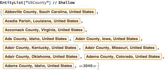
Now we inspect our entity store:

Back to GeoRegionValuePlot
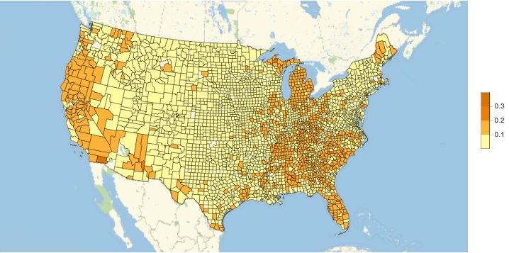
With the entity store in place we can now use GeoRegionValuePlot to plot our custom data like this:
GeoRegionValuePlot[EntityList[EntityClass["USCounty", "Mainland"]] -> "Unemployment"]
With a few options it looks almost the same as Bostock's map:
getColor[val_?NumericQ] := Which[
  0 < val < 0.01667, RGBColor[{247, 251, 255}/255],
  0.0166 < val < 0.0333, RGBColor[{222, 235, 247}/255],
  0.0333 < val < 0.05, RGBColor[{198, 219, 239}/255],
  0.05 < val < 0.0666, RGBColor[{158, 202, 225}/255],
  0.0666 < val < 0.0833, RGBColor[{107, 174, 214}/255],
  0.0833 < val < 0.1, RGBColor[{66, 146, 198}/255],
  0.1 < val < 0.1166, RGBColor[{33, 113, 181}/255],
  0.1166 < val < 0.1333, RGBColor[{8, 81, 156}/255],
  0.1333 < val < 0.15, RGBColor[{8, 48, 107}/255],
  True, RGBColor[{8, 48, 107}/255]
  ]
getColor[val_] := RGBColor[{8, 48, 107}/255]

mainland = GeoRegionValuePlot[
  EntityList[EntityClass["USCounty", "Mainland"]] -> "Unemployment",
  ColorFunction -> getColor,
  ColorFunctionScaling -> False,
  PlotLegends -> None,
  PlotStyle -> Directive[EdgeForm[None]],
  GeoBackground -> None,
  GeoProjection -> {
    "LambertAzimuthal",
    "Centering" -> GeoPosition[{30, -195/2}]
    },
  PlotRange -> {{-0.37, 0.38}, {-0.13, 0.38}},
  ImageSize -> 660
  ]
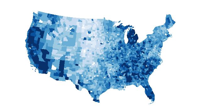
There are a few white counties here which are missing because they don't have the "FIPSCode" property. In my original version of this post over at Mathematica.StackExchange I used an external source for FIPS codes because at that time counties either did not have them or they were incorrect. Now that they are mostly correct I think that the added elegance of not having to use an external data source is preferred.
The last details
We now add Alaska and Hawaii:
getPolygon[entity_] := {
  GeoStyling[None],
  getColor[entity["Unemployment"]], Polygon[entity]
  }

alaska = GeoGraphics[
   getPolygon /@ EntityList[EntityClass["USCounty", "Alaska"]],
   GeoBackground -> None
   ];
hawaii = GeoGraphics[
   getPolygon /@ EntityList[EntityClass["USCounty", "Hawaii"]],
   GeoBackground -> None
   ];

map = Show[
  mainland,
  GeoGraphics[{
    Inset[alaska, {-0.3, -0.06}, {0, 0}, 0.3],
    Inset[hawaii, {-0.15, -0.06}, {0.1569, -0.0436}, 0.3]
    }]
  ]

We can see Hawaii, but unfortunately no county entities for Alaskan counties have FIPS codes in them, so Alaska has disappeared.
To add the borderlines I first make a black and white mask, where states are black and the background is white. The state borderlines that I want to draw are white as well; I then use ImageAdd to put the images together. The counties will be unaffected because we'll only be adding black to them, except for on the borderlines. In principle, I could add the GeoRegionValuePlot to the GeoGraphics with Hawaii, but I use GeoGraphics for both to ensure matching image padding.
states = Cases[
   EntityList@
    Entity["AdministrativeDivision", {"Country" ->
       Entity["Country", "UnitedStates"]}],
   Entity[_, {_, _}]
   ];

alaska = GeoGraphics[
   Polygon /@ EntityList[EntityClass["USCounty", "Alaska"]],
   GeoBackground -> None
   ];
hawaii = GeoGraphics[
   Polygon /@ EntityList[EntityClass["USCounty", "Hawaii"]],
   GeoBackground -> None
   ];

map = GeoGraphics[{
    getPolygon /@ EntityList[EntityClass["USCounty", "Mainland"]],
    Inset[alaska, {-0.3, -0.06}, {0, 0}, 0.3],
    Inset[hawaii, {-0.15, -0.06}, {0.1569, -0.0436}, 0.3]
    },
   GeoBackground -> None,
   GeoProjection -> {
     "LambertAzimuthal",
     "Centering" -> GeoPosition[{30, -195/2}]
     },
   PlotRange -> {{-0.37, 0.38}, {-0.13, 0.38}},
   ImageSize -> 1000
   ];

borders = GeoGraphics[{
    FaceForm[Black],
    EdgeForm[White],
    GeoStyling[None],
    Polygon /@ states,
    Inset[alaska, {-0.3, -0.06}, {0, 0}, 0.3],
    Inset[hawaii, {-0.15, -0.06}, {0.1569, -0.0436}, 0.3]},
   GeoBackground -> None,
   GeoProjection -> {
     "LambertAzimuthal",
     "Centering" -> GeoPosition[{30, -195/2}]
     },
   PlotRange -> {{-0.37, 0.38}, {-0.13, 0.38}},
   ImageSize -> 660
   ];

ImageAdd[map, borders]
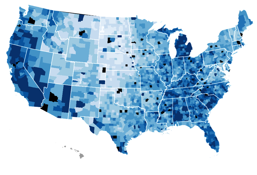
With all FIPS codes
When I used an external source for FIPS codes I had FIPS codes for all the counties. Here is an image which shows what the picture looks like then. Hopefully FIPS codes for the remaining counties will be added to the built-in knowledgebase in the future.
