Introduction
Correlation and covariance matrices are widely used objects in multivariate statistics and multi-dimensional process modelling. As such they represent one of the best known form used to determine dependency structure for linearly associated random variables.
Correlation plays important role in many statistical models and data analysis. Regression is one of them. Given the nature and importance of correlation in multivariate setting, its calculation and broader definition in the matrix context is a subjects of specific tests that prove the validity of construction arguments.

The appropriateness of correlation matrix for deeper statistical modelling is determined through consistency. Consistency of matrix looks into certain attributes that prove matrix usability for transformation and decomposition. For correlation and covariance matrices the consistency is usually measured through positive definiteness.
Positive definite and semi-definite matrices
Matrix positivity can be defined in different ways. When the matrix is real and symmetric, then the condition for positive definiteness can be simply expressed as A x.x >0 (for positive) and A x.x >= 0 (for semi-definite) for real matrix A and any vector x with real components.
The dot product condition of A x and x has also practical geometric representation, for every x, the angle between A x and x cannot exceed $\pi/2$. This is due to $\left< A x, x\right> = \left\|Ax\right\| \left\|x\right\| Cos\theta$ which implies $Cos\theta>0$.
When matrix is symmetric, the condition for positive definiteness / semi-definiteness resides on its eigenvalues. Symmetric matrix is positive definite (semi-definite) iff its eigenvalues are strictly positive (non-negative). Matrix positiveness is also related to matrix determinant. If the matrix is positive definite / semi-definite, determinant is always positive. This means that so a positive definite matrix is always nonsingular.
Why is this important? General least squares estimation and related regression methods reside on matrix invention. This in turn requires division by matrix determinant. When matrix is singular, then invention involves division by zero, which is undefined.
Causes of non-positivity of correlation matrices
There are number of reasons why correlation matrices can become non-positive.The most common cases point at the quality' of underlying data:
- Strong linear dependency amongst the data
- Errors in underlying data that prevent computation of covariances
- Excessive variations in sampling data
- Missing data with inconsistent replacements
- Presence of constant values
Why correlation matrices have to be positive
These is a sound theoretical argument showing why real correlation matrices have to be positive (semi) definite. Consider a number of n x m real data observation in the X set 
We standardise the data with Subscript[[Mu], 1] being mean and Subscript[[Sigma], 1] being standard deviation for series 1, Subscript[[Mu], 2] and Subscript[[Sigma], 2] for series 2 etc. We can then create new set of standardised series as follows: 
We can then create the correlation matrix C as follows: C = Subsuperscript[X, S, T] . Subscript[X, S] where superscript T denotes transpose.
From the definition of semi-definite positiveness of a matrix above, we know that real matrix M is positive semi-definite if for there is no vector z such that z^T M z <=0.
Let's now assume that our correlation matrix C is NOT positive semi-definite. Then, there must exist vector [Theta] that makes [Theta]'.C[Theta] <=0. We can write [Theta]^''C [Theta] as [[Theta]^' Subsuperscript[X, S, T] Subscript[X, S] [Theta]] or simply as ([Subscript[X, S][Theta]]])^T [Subscript[X, S] [Theta]]. We can write this product simply as Subsuperscript[[Lambda], 1, 2]+ Subsuperscript[[Lambda], 2, 2] + Subsuperscript[[Lambda], 3, 2].... Subsuperscript[[Lambda], n, 2] where [Lambda] = Subscript[X, S] [Theta]. This shows that [Theta]^T C [Theta] is merely a sum of squared variables, and as such cannot be negative. In view of the above, we can conclude that the correlation or covariance matrix by construction argument must be positive (semi)- definite. The statement is actually true for any matrix that can be written in the U^T U form.
Strategy for matrix correction
When correlation matrix is not positive semidefinite, we can apply simple correction technique to turn it into positive domain. The method of 'normalised shifts' guarantees conversion with output that can be used in chain calculation.
Mathematica implementation of this correction strategy is quick and efficient:
- Calculate the eigenvalues of the original matrix and get its lowest values
- Subtract this value from the matrix diagonal
- Normalise the result by the complement of the original eigenvalue set
- Adjust the diagonals
Let's consider the following 5x5 correlation matrix in which the last diagonal element is by mistake entered as -1 instead of 1. This matrix is clearly invalid.
CM1 = {{1, 0.35, 0.201, -0.14, -0.33}, {0.35, 1, -0.11, -0.44,
    0.07}, {0.201, -0.11, 1, -0.22, 0.33}, {-0.14, -0.44, -0.22, 1,
    0.02}, {-0.33, 0.07, 0.33, 0.02, -1}};
CM1 // MatrixForm
m = Dimensions[CM1][[1]];
PositiveDefiniteMatrixQ[CM1]

We now employ the 'correction algorithm' described above that converts the matrix into valid correlation matrix. We check this with Mathematica's testing function:
EvMin = Eigenvalues[CM1] // Min;
EvMin2 = Min[EvMin, 0];
EvIdm =  EvMin2 IdentityMatrix[m];
AdjCM = (CM1 - EvIdm)/(1 - EvMin2);
AdjCM = ReplacePart[AdjCM, {i_, i_} -> 1];
AdjCM // MatrixForm
PositiveDefiniteMatrixQ[AdjCM]

We now use the corrected correlation matrix to create the covariance matrix we intend to use in building multi-dimensional stochastic process:
VOL[n_, min_, max_] := RandomReal[{min, max}, n];
vl = VOL[m, 0.025, 0.05];
covM = Transpose[vl Transpose[vl AdjCM]];
covM // MatrixForm
PositiveDefiniteMatrixQ[covM]

Multi-dimensional Brownian Bridge Process
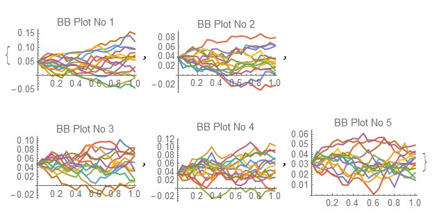
We can now apply the corrected matrix output to build 5-dimensional correlated Brownian Bridge [BB] process. Ito Process requires the covariance matrix to be explicitly positive definite.
We first defined the drift parameters for the BB process:
xtvar = Table[vars[[i]][t], {i, m}];
vars = Table[Symbol["x" <> ToString[i]], {i, m}]; tvar =
 Table[Symbol["t" <> ToString[i]], {i, m}]; lab =
 Table["BB Plot No " <> ToString[i], {i, m}];
bbdrift = (vars - xtvar)/(1 - tvar)         (*this is the drift denition of the BB *)

We then randomise the initial values and build the correlated BB process with the covariance matrix
iv = RandomReal[{0.02, 0.05}, m];
ip2 = ItoProcess[{bbdrift, IdentityMatrix[m]}, {vars, iv}, t, covM];
ProcessParameterQ[ip2]
True
We can now visualise the correlated BB processes
SeedRandom[Method -> "MersenneTwister"] ;
path2 = RandomFunction[ip2, {0, 1, 0.05}, 15,
  Method -> "StochasticRungeKutta"]; Evaluate@
 Table[ListLinePlot[path2["PathComponent", i], PlotRange -> All,
   PlotLabel -> lab[[i]], ImageSize -> 150], {i, m}]

Conclusion
The correction method for the correlation matrices may not be ideal in every instance, but it serves the purpose of adjusting the input matrix when further use of matrix requires strict matrix positivity. The larger the input 'error' the larger the potential deviation of the original matrix relative to the corrected one. if large errors in the input matrix are encountered, further examination of the adjusted matrix is advisable, such that the matrix definition still serves its purpose.
 Attachments: