I am very interested in your subject of chaos and the double pendulum. Your implementation with OOP was a surprise but I figured it out and I was able to learn a lot about UpValues, Upset, DelayedUpset etc...
However, I do not understand what is the exact advantage of using your OOP paradigm. I did the same using ParametricNDSolve and implemented your formulas without any problem.
Manipulate[
Quiet@Module[{T1, T2, V1, V2, L, lkeq,
ans, \[Theta]1Eff, \[Theta]2Eff, pendulum, butterfly, g = 9.8,
m = 1, r1 = 1, r2 = 0.5},
SeedRandom[13];
(*Lagrangian setup*)
T1 = 1/2 m*r1^2*\[Theta]1'[t]^2;
V1 = -m*g*r1*Cos[\[Theta]1[t]];
T2 = 1/
2 m*(r1^2*\[Theta]1'[t]^2 + r2^2*\[Theta]2'[t]^2 +
2 r1*r2*\[Theta]1'[t]*\[Theta]2'[t]*r1*r2*
Cos[\[Theta]1[t] - \[Theta]2[t]]);
V2 = -m*g*(r1*Cos[\[Theta]1[t]] + r2*Cos[\[Theta]2[t]]);
L = T1 + T2 - (V1 + V2);
(*Lagrange equation of motion*)
lkeq = {D[D[L, \[Theta]1'[t]], t] - D[L, \[Theta]1[t]] == 0,
D[D[L, \[Theta]2'[t]], t] - D[L, \[Theta]2[t]] == 0};
(*Numerical solve parametric differential equation:
parameter is the initial angular displacement increment*)
ans = ParametricNDSolve[{lkeq, {\[Theta]1[0] ==
th1 + \[Epsilon], \[Theta]2[0] ==
th2 + \[Epsilon], \[Theta]1'[0] == 0, \[Theta]2'[0] ==
0}}, {\[Theta]1, \[Theta]2}, {t, 0, time}, {\[Epsilon]},
MaxSteps -> \[Infinity], PrecisionGoal -> \[Infinity]];
\[Theta]1Eff[\[Epsilon]_, tr_] := \[Theta]1[\[Epsilon]][tr] /.
ans;
\[Theta]2Eff[\[Epsilon]_, tr_] := \[Theta]2[\[Epsilon]][tr] /. ans;
butterfly = 10^-pwr;
pendulum[\[Epsilon]_, col_: Black] := {col,
Line[{{0,
0}, {r1*Sin[\[Theta]1Eff[\[Epsilon], tr]], -r1*
Cos[\[Theta]1Eff[\[Epsilon], tr]]}}],
Line[{{r1*Sin[\[Theta]1Eff[\[Epsilon], tr]], -r1*
Cos[\[Theta]1Eff[\[Epsilon], tr]]}, {(r1*
Sin[\[Theta]1Eff[\[Epsilon], tr]] +
r2*Sin[\[Theta]2Eff[\[Epsilon], tr]]), (-r1*
Cos[\[Theta]1Eff[\[Epsilon], tr]] -
r2*Cos[\[Theta]2Eff[\[Epsilon], tr]])}}]};
(*-----graphics display--------*)
Graphics[
Map[pendulum[butterfly*#1, Hue[#1]] &, RandomReal[{-1, 1}, n]],
PlotRange -> {{-1.8, 1.8}, {-1.8, 1.8}}]],
(*-----controls--------*)
{{tr, 0, Style["time", 12]}, 0, time,
Animator, AnimationRunning -> False, AnimationRepetitions -> 1,
AnimationRate -> .025},
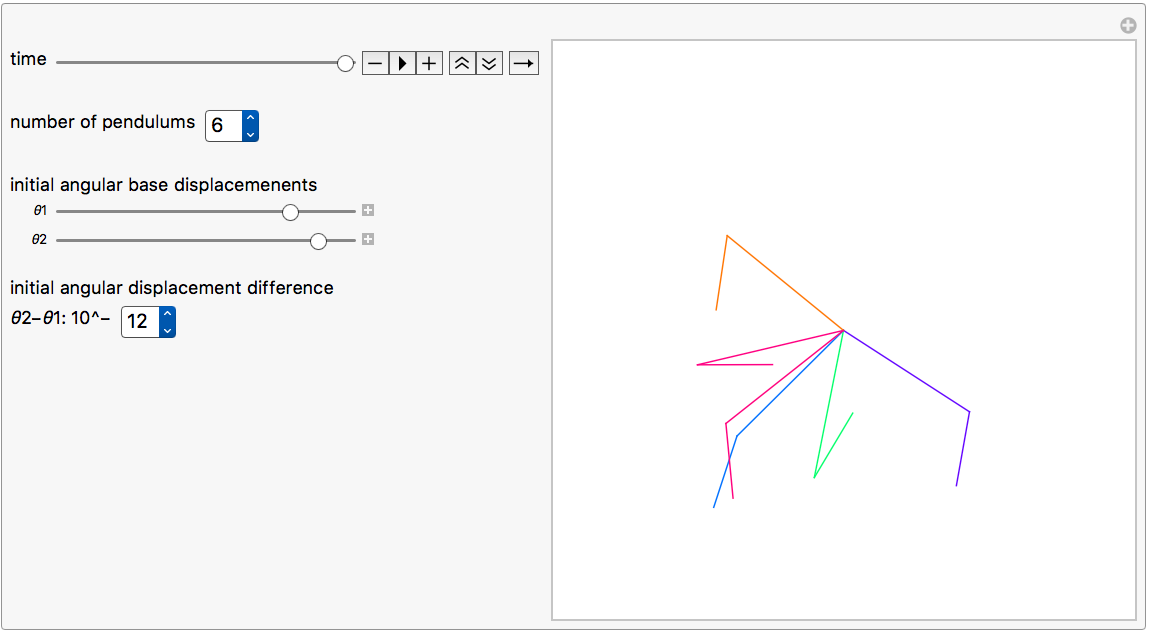
Row[{Style["\nnumber of pendulums", 12],
Control[{{n, 6, ""}, Range[12]}]}],
Style["\ninitial angular base displacemenents",
12], {{th1, 2., "\[Theta]1"}, -3.14,
3.14}, {{th2, 2.5, "\[Theta]2"}, -3.14, 3.14},
Row[{Style[
"\ninitial angular displacement difference\n\[Theta]2-\[Theta]1: \
10^-", 12], Control[{{pwr, 12, ""}, Range[3, 16]}]}], {{time, 50},
None},
(*-----options--------*)
TrackedSymbols :> Manipulate,
AutorunSequencing -> {}, ControlPlacement -> Left]
I further more could introduce a variable number of pendulums and a variable "butterfly" value. All this using plain functional programming. Your method is very elegant and smart but what exactly can one do more,faster or better with OOP?