Introduction
In general the period of an oscillation can depend on a variable parameter such as energy, here $\alpha$. Then two distinct oscillators of variable energy are called isoperiodic whenever periods equal for all values of $\alpha$ : $T_{1}(\alpha)=T_{2}(\alpha)$. Even in the simple setting of Hamiltonian oscillation, there are a wide range of possibilities as explored in the following Demonstration:
http://demonstrations.wolfram.com/IsoperiodicPotentialsViaSeriesExpansion
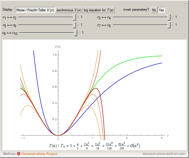
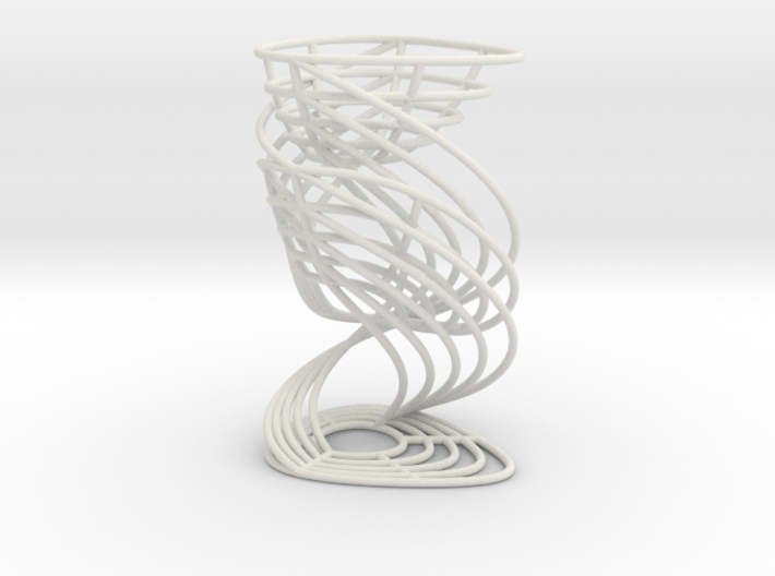
This demonstration focuses solely on construction of isoperiodic potentials, which are curves in two dimensions. Exact solutions of the time-dependent oscillation make for beautiful geometry in a three-dimensional space where time goes along the vertical, above the horizontal plane, phase space. Using the Morse and PöschlTeller example, as in the demonstration above, we construct the following models and export to Shapeways:
https://www.shapeways.com/product/GXBPX8F24/morse-oscillator-time-helices?optionId=62983286
https://www.shapeways.com/product/BB74864YX/poschl-teller-oscillator-time-helices?optionId=62983299
When the printed models stand side-by-side on a flat surface, the upper-most level sets are at equal heights, a stunning and tangible demonstration of isoperiodicity. Contrasting demonstration with models, it's rewarding to imagine that the continuous deformation of potentials implies a continuous deformation between the two models. Expect to hear more about symmetry breaking in the near future, but for now we will discuss an example where symmetry is added rather than broken !
Simple Pendulum ( Again )
First we construct the phase space trajectory by applying series inversion as in numerous previous references ( Cf. W.C. 1 , W.C. 2 ). We then run a couple of validation test to make sure the general primitives look roughly okay:
vSet[n_, m_] :=
 Map[Range[n] /. Append[Rule @@ # & /@ Tally[#], x_Integer :> 0] &,
  DeleteCases[
   Select[IntegerPartitions[n + m], Length[#] > m - 1 &], {n + 1,
    1 ...}]]

GExp[n_] := y*Total[y^# g[#] & /@ Range[0, n - 1]]

gCalc[0, _] = 1;
gCalc[n_, m_] := With[{vs = vSet[n, m]},
  Total@ReplaceAll[Times[-1/m, Multinomial @@ #, c[Total[#] - m],
       Times @@ Power[gSet[#] & /@ Range[0, n - 1], #]] & /@ vs,
    {c[0] -> 1}]]

MultinomialExpand[n_, m_] := Module[{},
  Clear@gSet; Set[gSet[#], Expand@gCalc[#, m]] & /@ Range[0, n - 1];
  Expand[GExp[n + 1] /. g[n2_] :> gCalc[n2, m]]]

\[Psi]Test = MultinomialExpand[10, 2] /. c[x_] :> c[x] Q^(x + 2);

TrigReduce[Normal@Series[
   (p^2 + q^2 + Total[c[#] q^(# + 2) & /@ Range[5] ]
      ) /. {p -> \[Psi]Test Sin[\[Phi]], q -> \[Psi]Test Cos[\[Phi]]
      } /. Q -> Cos[\[Phi]], {y, 0, 5}]]

SameQ[
 With[{exp = TrigReduce[Normal@Series[
        -Q D[\[Psi]Test, Q]/\[Psi]Test - 1,
        {y, 0, 2}] /. Q -> Cos[\[Phi]]]},
  Expand[Coefficient[exp, y, #] & /@ Range[0, 2]]],
 With[{exp = TrigReduce[Normal@Series[
        D[
          Expand[-(1/2)*\[Psi]Test^2 /.
            y -> (2 \[Alpha])^(1/2)], \[Alpha]] /. \[Alpha] -> (1/
             2) y^2,
        {y, 0, 2}] /. Q -> Cos[\[Phi]]]},
  Expand[Coefficient[exp, y, #] & /@ Range[0, 2]]]]
The first prints $y^2$, suggesting the correct series inversion. The second prints "True" suggesting that the time-dependence is calculated correctly.
All that remains is to fill in values for the expansion coefficients, and then to plot. Here we limit ourselves to half the total energy range:
\[Psi]Pendulum = Sqrt[2 \[Alpha]] Expand[
    (MultinomialExpand[20, 2] /. c[x_] :> c[x] Q^(x + 2) /.
         c[x_ /; OddQ[x]] :> 0 /. {c[2] -> (-1/12), c[4] -> 1/360,
         c[6] -> (-1/20160)} /. y -> Sqrt[4 \[Alpha]])/
     Sqrt[4 \[Alpha]]] /. \[Alpha]^n_ /; n > 3 :> 0

dt = TrigReduce[
    D[Expand[(1/2)*\[Psi]Pendulum^2], \[Alpha]] /.
     Q -> Cos[\[Phi]]] /. \[Alpha]^n_ /; n > 5 :> 0;

t[\[Phi]1_, \[Phi]2_] :=
 Expand[(1/2/Pi) Integrate[dt, {\[Phi], \[Phi]1, \[Phi]2}]]

tA\[Phi] = t[Pi/2, Pi/2 + \[Phi]];

tB\[Phi] = t[3 Pi/2, 3 Pi/2 + \[Phi]];

tC\[Phi] = t[Pi/2 + \[Phi], \[Phi] + Pi + Pi/2];

tB\[Phi] + tA\[Phi] /. {\[Phi] -> Pi}


PST = (\[Psi]Pendulum /. Q -> Cos[\[Phi] + Pi/2]) {Cos[\[Phi] + Pi/2],
     Sin[\[Phi] + Pi/2], 0};
PST2 = (\[Psi]Pendulum /.
     Q -> Cos[\[Phi] + Pi/2 + Pi]) {Cos[\[Phi] + Pi/2 + Pi],
    Sin[\[Phi] + Pi/2 + Pi], 0};

DoubleHelixPendulum = Show[
  ParametricPlot3D[Evaluate[
    Plus[PST, {0, 0, -2 tA\[Phi]}] /. \[Alpha] -> .5 #/5 & /@
     Range[5]],
   {\[Phi], 0, -2 Pi}, PlotStyle -> Tube[1/32], PlotPoints -> 100],
  ParametricPlot3D[Evaluate[
    Plus[PST2, {0, 0, -2 tB\[Phi]}] /. \[Alpha] -> .5 #/5 & /@
     Range[5]],
   {\[Phi], 0, -2 Pi}, PlotStyle -> Tube[1/32], PlotPoints -> 100],
  ParametricPlot3D[Evaluate[
    Plus[PST, {0, 0, 2 tC\[Phi]}] /. \[Alpha] -> .5 #/5 & /@ Range[5]],
   {\[Phi], 0, 1.1 2 Pi}, PlotStyle -> Tube[1/32], PlotPoints -> 100],

  ParametricPlot3D[Evaluate[
    Plus[PST2, {0, 0,
         2 tB\[Phi] /. \[Phi] -> 2 Pi}] /. \[Alpha] -> .5 #/5 & /@
     Range[5]],
   {\[Phi], 0, -1.1 2 Pi}, PlotStyle -> Tube[1/32], PlotPoints -> 100],
  ParametricPlot3D[Evaluate[
    Plus[PST2, {0, 0,
         2 tB\[Phi] /. \[Phi] -> 0}] /. \[Alpha] -> .5 #/5 & /@
     Range[5]],
   {\[Phi], 0, -1.1 2 Pi}, PlotStyle -> Tube[1/32], PlotPoints -> 100],
  ParametricPlot3D[Evaluate[
    Plus[PST2, {0, 0, 2 tB\[Phi] /. \[Phi] -> 0}] /. \[Phi] ->
        2 Pi #/6 & /@ Range[6]],
   {\[Alpha], .1, 0.5}, PlotStyle -> Tube[1/32], PlotPoints -> 100],

  ParametricPlot3D[Evaluate[
    Plus[PST, {0, 0, 2 tC\[Phi]}] /. \[Phi] -> 2 Pi #/6 & /@ Range[6]],
   {\[Alpha], .1, 0.5}, PlotStyle -> Tube[1/32], PlotPoints -> 100],

  ParametricPlot3D[Evaluate[
    Plus[PST2, {0, 0, 2 tB\[Phi] /. \[Phi] -> 2 Pi}] /. \[Phi] ->
        2 Pi #/6 & /@ Range[6]],
   {\[Alpha], .1, 0.5}, PlotStyle -> Tube[1/32], PlotPoints -> 100],

  Boxed -> False, Axes -> False, PlotRange -> All, ImageSize -> 300
  ]
This model can be saved as an ".stl" file and exported directly to shapeways.
Shapeways: Simple Pendulum Time Helices
Edward's Curve
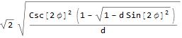
As recently announced on seqfans, it's relatively easy to apply polar coordinates in an analysis of the Edward's Curve ( Cf. Edwards & Bernstein & Lange ), and this approach readily yields a simple exact form for the "time dependence" of the addition rules. First we calculate a radius function for the genus-one solution:
Edwards = x^2 + y^2 - (1 + d x^2 y^2);
r[\[Phi]_] :=  Sqrt[(1 - Sqrt[1 - d Sin[2 \[Phi]]^2]) 2  Csc[2 \[Phi]]^2/d]
r[\[Phi]]
And check this:
TrigReduce[ Edwards /. {x -> r[\[Phi]] Cos[\[Phi]], y -> r[\[Phi]] Sin[\[Phi]]}]
Yields Zero, as necessary. TrigReduce can be replaced by a set of replacement rules. Next we write the addition rule in the form of a tangent function,
Tan\[Phi]3[\[Phi]1_, 0] := Tan[\[Phi]1]
Tan\[Phi]3[\[Phi]1_, \[Phi]2_] :=  Tan[\[Phi]1 + \[Phi]2] (1 - d z)/(1 + d z) /.
  z -> r[\[Phi]1]^2 r[\[Phi]2]^2 Cos[\[Phi]1] Sin[\[Phi]1] Cos[\[Phi]2] Sin[\[Phi]2]
And calculate the derivative
\[Phi]dot = Times[
  Normal@Series[ Tan\[Phi]3[\[Phi],   \[Omega]dt], {\[Omega]dt, 0, 1}] -  Tan\[Phi]3[\[Phi], 0],
  Cos[\[Phi]]^2/\[Omega]dt  ]
d\[Phi]/TrigReduce[Expand[\[Phi]dot]]
The closed form result is ,
$$\omega \; dt = \frac{d\phi}{\sqrt{1-d \sin^2(2\phi)}} = \frac{d\phi}{\sqrt{1-4 \;d \big( \sin(\phi)\cos(\phi)\big)^2}} .$$
Clearly the complete elliptic integral of the first kind is given by any integral of the form
$$K(d) \propto \frac{1}{2\pi} \int_{0}^{2\pi} \frac{d\phi}{\sqrt{1-d \sin^2(n\;\phi)}}, $$
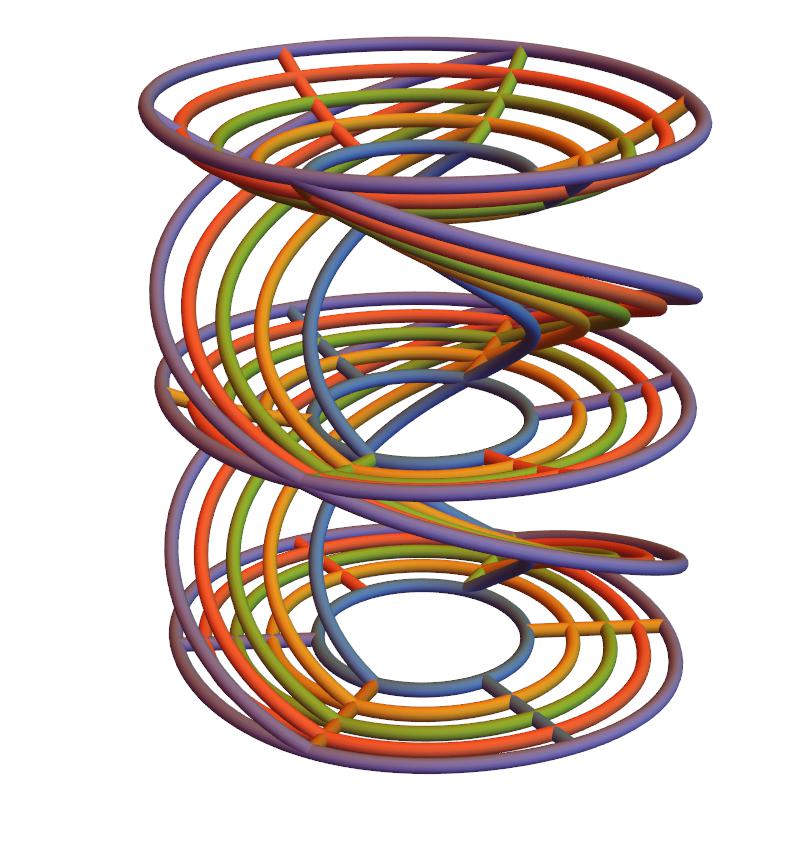
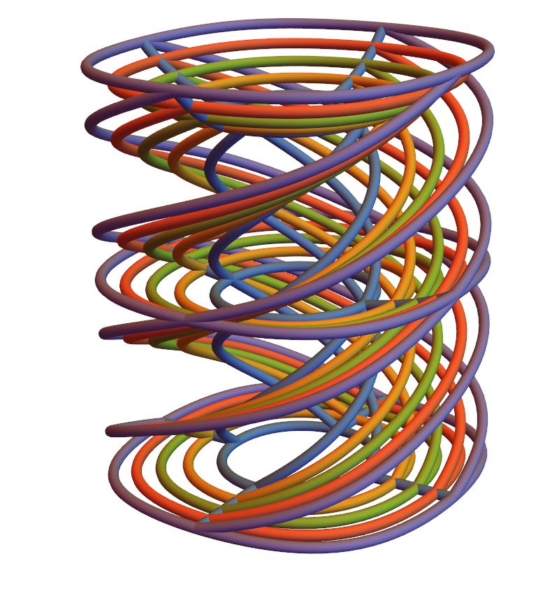
with integer $n$. As is well known the pendulum has $n=1$, and we see here that Edward's curve has $n=2$, proving the two systems are isoperiodic. Let's now exploit the square symmetry of Edward's curve by making a quadruple-helix, 3D-printable Model.
First we expand the radius to avoid singular points, and integrate the time dependence ( this is done naively, and could be optimized with a little more effort ),
rEdwards = Normal[Series[Sqrt[2 d] r[\[Phi]0], {d, 0, 20}]];
dt = 1/Sqrt[Expand[1 - 4 d x^2]] d\[Phi]
t = 1/2/Pi Integrate[ Evaluate[  Expand[TrigReduce[   Normal@Series[dt, {d, 0, 20}] /.
         x -> Cos[\[Phi]] Sin[\[Phi]]]/d\[Phi]]], {\[Phi],   Pi, \[Phi]0}];
The extra factor of $\sqrt{d}$ corresponds to a coordinate change where Edward's equation takes a form $d = x^2+y^2-x^2y^2$, which allows us to plot the time spirals,
EdwardsQuadrupleHelix = Show[
  Function[{a},
    ParametricPlot3D[
     Evaluate[{rEdwards Cos[\[Phi]0 + Pi/2 a],
          rEdwards Sin[\[Phi]0 + Pi/2 a], 2 t} /. d -> #/10 & /@
       Range[5]], {\[Phi]0, Pi, 3 Pi}, PlotStyle -> Tube[1/32],
     PlotPoints -> 100]
    ] /@ Range[0, 3],

  Function[{a},
    ParametricPlot3D[
     Evaluate[{rEdwards Cos[\[Phi]0 + Pi/2 a],
        rEdwards Sin[\[Phi]0 + Pi/2 a], 2 t} /. \[Phi]0 -> Pi], {d,
      0.1, .5}, PlotStyle -> Tube[1/32], PlotPoints -> 100]
    ] /@ Range[0, 3],

  Function[{a},
    ParametricPlot3D[
     Evaluate[{rEdwards Cos[\[Phi]0 + Pi/2 a],
        rEdwards Sin[\[Phi]0 + Pi/2 a], 2 t} /. \[Phi]0 -> 2 Pi], {d,
      0.1, .5}, PlotStyle -> Tube[1/32], PlotPoints -> 100]
    ] /@ Range[0, 3],

  Function[{a},
    ParametricPlot3D[
     Evaluate[{rEdwards Cos[\[Phi]0 + Pi/2 a],
        rEdwards  Sin[\[Phi]0 + Pi/2 a], 2 t} /. \[Phi]0 -> 3 Pi], {d,
       0.1, .5}, PlotStyle -> Tube[1/32], PlotPoints -> 100]
    ] /@ Range[0, 3],


  ParametricPlot3D[
   Evaluate[{rEdwards Cos[\[Phi]0 + Pi], rEdwards Sin[\[Phi]0 + Pi],
        2 t /. \[Phi]0 -> Pi} /. d -> #/10 & /@ Range[5]], {\[Phi]0,
    Pi, 3 Pi}, PlotStyle -> Tube[1/32], PlotPoints -> 100],
  ParametricPlot3D[
   Evaluate[{rEdwards Cos[\[Phi]0 + Pi], rEdwards Sin[\[Phi]0 + Pi],
        2 t /. \[Phi]0 -> 2 Pi} /. d -> #/10 & /@
     Range[5]], {\[Phi]0, Pi, 3 Pi}, PlotStyle -> Tube[1/32],
   PlotPoints -> 100],
  ParametricPlot3D[
   Evaluate[{rEdwards Cos[\[Phi]0 + Pi], rEdwards Sin[\[Phi]0 + Pi],
        2 t /. \[Phi]0 -> 3 Pi} /. d -> #/10 & /@
     Range[5]], {\[Phi]0, Pi, 3 Pi}, PlotStyle -> Tube[1/32],
   PlotPoints -> 100]

  , PlotRange -> All, Boxed -> False, Axes -> False, ImageSize -> 800
  ]
Again, can be exported directly to shapeways. Finally let's take a closer look at isoperiodicity, by comparing the upper-most level sets,
Show[Function[{a},
   ParametricPlot3D[
    Evaluate[{rEdwards Cos[\[Phi]0 + Pi/2 a],
       rEdwards  Sin[\[Phi]0 + Pi/2 a], 2 t} /. \[Phi]0 -> 3 Pi], {d,
     0.1, .5}, PlotStyle -> Tube[1/32], PlotPoints -> 100]
   ] /@ Range[0, 3],
 ParametricPlot3D[
  Evaluate[{rEdwards Cos[\[Phi]0 + Pi], rEdwards Sin[\[Phi]0 + Pi],
       2 t /. \[Phi]0 -> 3 Pi} /. d -> #/10 & /@ Range[5]], {\[Phi]0,
   Pi, 3 Pi}, PlotStyle -> Tube[1/32], PlotPoints -> 100],
 Show[ParametricPlot3D[Evaluate[
    Plus[PST2, {0, 0,
         2 tB\[Phi] /. \[Phi] -> 2 Pi}] /. \[Alpha] -> .5 #/5 & /@
     Range[5]],
   {\[Phi], 0, -1.1 2 Pi}, PlotStyle -> Tube[1/32], PlotPoints -> 100],
  ParametricPlot3D[Evaluate[
    Plus[PST2, {0, 0, 2 tB\[Phi] /. \[Phi] -> 2 Pi}] /. \[Phi] ->
        2 Pi #/6 & /@ Range[6]],
   {\[Alpha], .1, 0.5}, PlotStyle -> Tube[1/32], PlotPoints -> 100]],
 PlotRange -> All, Boxed -> False, Axes -> False, ImageSize -> 800
 ]
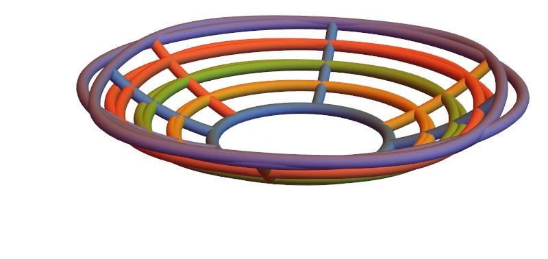
If you look closely, on the outermost trajectory, the effects of overly-liberal series truncation are narrowly observable. However, the physical scale for the error is about 1/100 of an inch, around the precision limit of the printer, so why worry?
Conclusion
We have shown that, with a little more work, computer-based calculus could be exported to a formal pen-and-paper proof of isoperiodicity between the simple pendulum and the Edward's Curve with addition rules. This is well demonstrated by the level sets of 3D printed models. Work is on-going regardless of anything else...


