Hello, I'm Selina Dasol Kim. As a student in Wolfram Alpha’s High School Summer Camp, I’ve had the opportunity to create a project based on my own interests—specifically, neuroscience! This project is an analysis of patch clamp recordings from rat neurons, specifically auditory cortex neurons in a live rat. Working with this type of data was novel experience for me, and I enjoyed it immensely. In this project, I identified spikes from the surrounding noise in electrophysiological data from neurons, and found out where these spikes are. This project could be used and tweaked to discover and plot other types of similar electrophysiological data.

I've attached a notebook with my code to this post.

Basic Neuroscience

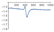
Neurons are the basic cells of the nervous system (the other major group of cells in this system, glia, support neurons in their work), and the communication between neurons, in the form of electrical signals, is the basis of all general functions of the brain. When neurons fire an electrical impulse, there is a rapid change in charge inside the cell–we can see this in the form of a spike in the image below. What my project does is find where the spikes are in the data and plot the data to emphasize them.

The Dataset

I’d like to thank CNCRS, which made this data available to me, and Anthony Zador's laboratory and Michael DeWeese of UC Berkeley, from whom this data is from; I did not play any role in gathering this data and simply analyzed it. The data was organized into lists of data points that could be plotted to form a graph of the data. In such a visual format, there were clearly two main features: spikes from the specific neuron and noise from surrounding neurons. For this project, a data file was partitioned into 100-point lists that would be used for training and classification.

   datafile = Import["path_to_file", "Data"]
   data = Flatten[
      Partition[datafile[[2, #]], 100] & /@ Range[Length@ac2data1[[2]]], 
      1]

Supervised Classification

After obtaining our data we were able to begin to train a classifier on the dataset. Since attempts to classify each list of data points were unsuccessful due to inherent relationships between numbers, we plotted each 100 point in separate graphs to train our classifier on images.

Images of partitioned data

  test = 
       With[fullMin=Min[Flatten[data]], fullMax=Max[Flatten[data]],
        (ListLinePlot[data[[#]], 
          PlotRange -> {All, {fullMin, fullMax}}] )]& /@ 
        Range[Length@data];  

Forming a training and testing set

After plotting the partitioned data file, I labelled each as either a “spike” or “noise” through a metric based on anomaly detection. To do so, I first took the mean of a list; “spikes” would then be lists with points outside a certain range from the mean.

trainingSet = 
    With[{cutoff = .02, trainingdata = data[[#]], fullmin = Min[Flatten[data]], fullmax=Max[Flatten[data]]}, 
      (*set symbols: cut off=how far the points have to be from the mean for the list to be a spike
      trainingdata=the specific list being analyzed
      fullmin = minimum of entire dataset, to determine the range of the graph so that each graph is on an equal scale
      fullmax = maximum of entire dataset, used in the same manner as fullmin*)

      (ListLinePlot[data[[#]], Axes -> False, PlotRange -> {Automatic, {fullmin, fullmax}}]  (*the list is plotted here; there 
      are no axes, and the domain is based on individual lists while the range is based on the minimum and maximum of 
       the entire dataset *)
         -> 
         If[(Abs[Min[trainingdata] - Mean[trainingdata]] >  cutoff) ||
            (Abs[Max[trainingdata] - Mean[trainingdata]] > cutoff), (*if either extrema of the individual list is outside a certain range of the mean….*)
            "spike",  (* then the list is labelled a spike *)
            "noise"]) (* otherwise, the list is labelled as noise*)
       ] & /@ Range[2000] (*the first 2000 lists in the datasets are used in this piece of code*)

Classifying

Looking at the numbers of training cases available for each class, there is clearly a smaller number of "spikes" compared to "noise".

 (*Finding out how many spikes and noise there are in trainingSet -- notice the skewed training set*)
 Counts[trainingSet[[All, 2]]]
 "noise" -> 1863, "spike" -> 137

For classification, I took advantage of the Mathematica function “Classify[]”; additionally, I added “ClassPriors” since my dataset was skewed heavily to noise.

cF = Classify[trainingSet,  ClassPriors -> <|"noise" -> 1863/2000, "spike" -> 137/2000|>]

Testing and Plotting

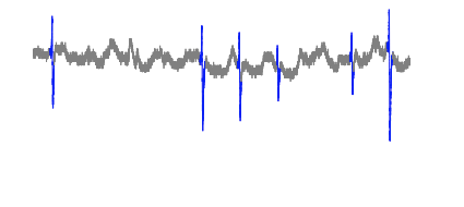
To visualize the data, I plotted “spike”-labelled lists in blue and “noise”-labelled lists in gray. Each individual data point was assigned to a color, based on what classification the data point’s list was in; for example, a data point that was in a list classified as "spike" would be blue, and so on for each point in that list.

foo = Flatten[With[{cutoff = .017, plotData = data[[#]]}, (*test has the plots of the dataset*) 
          If[(cF[ListLinePlot[plotData, Axes -> False, PlotRange -> {Automatic, {fullmin, fullmax}}]] == 
            "spike"), (*if the classifier deems the plot to be a spike…*)
            {Blue, #} & /@ plotData, (*then the points of this 100-point list are assigned to the color blue*)
            {Gray, #} & /@ plotData] (*otherwise, if the plot is considered to be noise, the points are assigned to the color gray*)
          ] & /@ Range[5000, 5500], 1]   

Then, appropriately colored lines were created between each data point.

(*Putting results of foo into correct format for the function Graphics...*)
lines =
  Flatten[List[foo[[#, 1]],
     Line[
      List[
       List[#, foo[[#, 2]]],
       List[# + 1, foo[[# + 1, 2]]]
       ]
      ]
     ] & /@ Range[Length@foo - 1], 1]

(*Plotting*)
Graphics[lines, 
 PlotRange -> {Automatic, {Min[data], Max[data]}}, AspectRatio -> 1] 

Images

As I created the training set, different cutoff points–on how far extremes of a 100-point list could be from the mean before the list would be labelled a "spike"–were used. For example, a cutoff point of 0.020, which I ended up using for my data set, would mean that the list would be labelled as a "spike" if the minimum or maximum of that list was at least 0.020 greater or less than the mean.

Cut off: 0.013

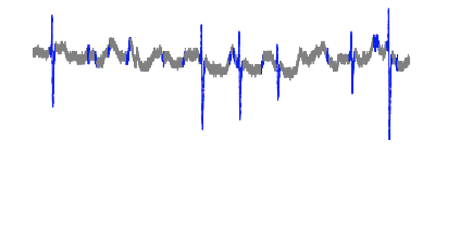
Zoomed in to another section of dataset:

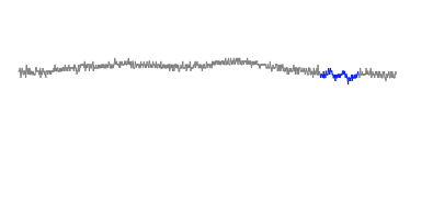
Cut off: 0.017

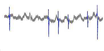
Cut off: 0.020

The plot looks extremely similar to that of 0.017, but this particular cut off point has less mistakes in other sections of the dataset.

Extensions

During my two weeks at the 2017 Wolfram Summer Camp, I learned a lot about using neural electrophysiological data; this project was a wonderful introduction for me in spike sorting. As I wasn't able to fully achieve all that I'd hoped to, I'll continue to work on refining and extending this project by exploring more effective methods of identifying spikes and working on classifying different kinds of spikes. While this current project focused on only a certain kind of spike, I'd like to extend the methods I use so that I can find and identify different spike patterns; I'd like to use other data as well.

Acknowledgments

Thank you to my mentor Rob Morris and the instructors at the Wolfram High School Summer Camp—these two weeks were an incredible experience for me. In addition, I'm extremely grateful to CNCRS for making this data available for me to use.

References

Deweese, Michael R.; Zador, Anthony M. (2011): Whole cell recordings from neurons in the primary auditory cortex of rat in response to pure tones of different frequency and amplitude, along with recordings of nearby local field potential (LFP). CRCNS.org. http://dx.doi.org/10.6080/K0G44N6R

Attachments: