First of all, I had my bracket in the wrong place because I wanted the first row to be the Beam Type and the second row to be the mode. I fixed this in the code below.
Next, I do not understand your approach for solving for the mode shapes -- you are setting the root finder for the eigenvalues at arbitrary spacing and this will not guaranty that you get a solution. I would use the formulas in a book such as Blevins:
Blevins, R.D., "Formulas for Natural Frequency and Mode Shape", Krieger Publishing Company, 2001. ISBN 9781575241845, Page 108-109.
What I would do: He gives an approximate formula for the eigenvalues -- use this for your starting value -- its real close. solve for the actual lambdas for each mode and then use the lambda for plotting in the beam equations provided. I do not understand your "f" equation. Is that a Taylor series for the actual equation? I am curious where that comes from.
(* Define some beam shape equations (from Blevins)*)
freeFreeShape[l_, x_] :=
Cosh[l*x] +
Cos[l*x] - (Cosh[l] - Cos[l])/(Sinh[l] - Sin[l])*(Sinh[l*x] +
Sin[l*x]);
freeSlidingShape[l_, x_] :=
Cosh[l*x] +
Cos[l*x] - (Sinh[l] - Sin[l])/(Cosh[l] + Cos[l])*(Sinh[l*x] +
Sin[l*x]);
clampedFreeShape[l_, x_] :=
Cosh[l*x] -
Cos[l*x] - (Sinh[l] - Sin[l])/(Cosh[l] + Cos[l])*(Sinh[l*x] -
Sin[l*x]);
freePinnedShape[l_, x_] :=
Cosh[l*x] +
Cos[l*x] - (Cosh[l] - Cos[l])/(Sinh[l] - Sin[l])*(Sinh[l*x] +
Sin[l*x]);
(* Define a DynamicModule to do the interaction *)
DynamicModule[{M =
100, lambdas, lambdaEqns, approxLambdas, n, beam = 1, ans,
modeshapes, i, maxCases = 4, maxModes = 10, lamValue},
(* Order in the following lists is Free-Free, Free-Sliding, \
Clamped-Free, Free-Pinned *)
(* List of equations for lambda (from \
Blevins) we will be finding the lamvalue that makes them zero later *)
lambdaEqns = {Cos[lamValue]*Cosh[lamValue] - 1,
Tan[lamValue] + Tanh[lamValue], Cos[lamValue]*Cosh[lamValue] + 1,
Tan[lamValue] - Tanh[lamValue]};
(* List of equations for approximate lambda (from Blevins) we will \
use these as starting guesses later *)
approxLambdas = {(2*i + 1) Pi/2., (4*i - 1) Pi/4., (2*i - 1) Pi/
2., (4*i - 1) Pi/4.};
(* Create a list of the solutions -- there are maxCases (I only did \
4 beam types so this is 4) lists each with the first maxModes lambdas*)
lambdas =
Table[lamValue /.
Table[FindRoot[
lambdaEqns[[indx]], {lamValue, approxLambdas[[indx]]},
WorkingPrecision -> 18], {i, maxModes}], {indx, maxCases}];
(* make a list of the functions so we can choose from them when \
plotting *)
modeshapes = {freeFreeShape, freeSlidingShape, clampedFreeShape,
freePinnedShape};
(* make a panel and plot things up *)
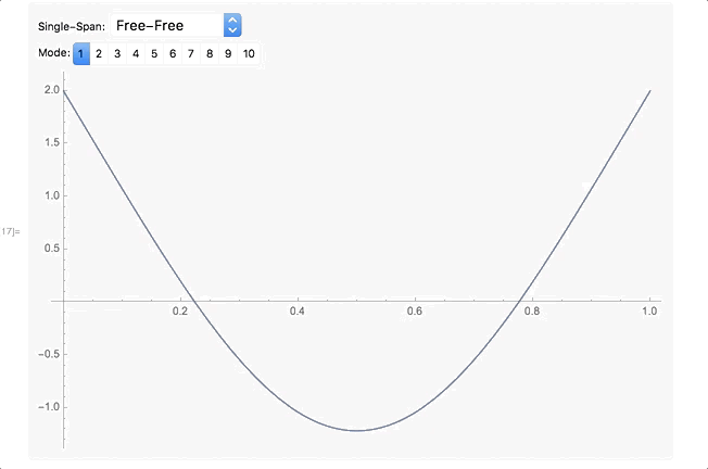
Panel[Column[{Row[{"Single-Span: ",
PopupMenu[
Dynamic[beam], {1 -> "Free-Free", 2 -> "Free-Sliding",
3 -> "Clamped-Free", 4 -> "Free-Pinned"}]}],
Row[{"Mode:", SetterBar[Dynamic[n], Range[maxModes]]}],
(*Dynamically choose a modeshape equation and apply it to two \
arguements -- the corresponding lambda by indexing into the lambda \
list first by beam, then by mode number, plot it in x *)
Dynamic[Plot[modeshapes[[beam]][lambdas[[beam, n]], x], {x, 0, 1},
ImageSize -> Large]]}]]]
I create a list of the functions to solve to get the eigenvalues (lambdas) for each beam type. Next create a list of the approximate lambda formulas so the guesses are very close. Next create a list of actual lambdas by solving the equation from the first list with the starting values from the second list. Next I would create a list of mode shape equations. When you choose a beam type, you choose a set of lambdas for that beam type and an equation for the beam shape. I put it together for a few beams -- you will need to add the rest. Note I defined the equations for the beam shapes outside of the Dynamic -- this was not necessary -- you could paste that block inside the DynamicModule before the line modeshapes = ... and make them local functions by adding them to the local variable list -- so they are not globally defined -- its up to you.
This is what it looks like:
Regards,
Neil


