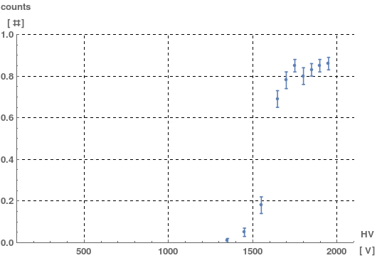
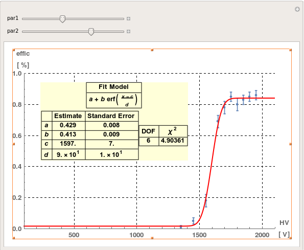
Hi everybody! I'd like to share the notebook i wrote for fitting experimental data (1-dimension) with a generic function. I've used it during the years at the Physics University to produce lab reports. I want to share it with the community and hear your opinions/advices/critics. I divided the code in section using comment line. For using/trying the notebook you just have to fill the section with the word "ENTRIES"

(I also attack the .nb file in this post because it's very more clear respect to see it here in the post)

(* ~~ENTRIES~~ In this section insert all your experimental data and the parameteres for the plot*)

datax = {1950, 1898, 1849, 1801, 1750, 1699, 1647, 1551, 1451, 1351};
datay = {0.86, 0.85, 0.83, 0.80, 0.85, 0.78, 0.69, 0.18, 0.05, 0.01};
erry = {0.03`, 0.03`, 0.03`, 0.04`, 0.03`, 0.04`, 0.04`, 0.04`, 0.02`,0.01`};
errx = {5, 5, 5, 5, 5, 5, 5, 5, 5, 5};
xmin = 100;
xmax = 2100;
ymin = 0;
ymax = 1;
xaxisname = "HV";
xaxisunit = "\n[V]";  (*use the ASCII \n if you want a newline*)
yaxisname = "counts";
yaxisunit = "\n[#]";


(*Elaboration for the plot of the with errors bars in order the check the data inserted in the previous section *)

s = erry;
numpt = Length[datax];
listdat = Table[{datax[[i]], datay[[i]]}, {i, numpt}];

listerr = 
  Table[{listdat[[i]], ErrorBar[{-s[[i]], s[[i]]}]}, {i, numpt}];
err = ErrorListPlot[{listerr}, 
  AxesLabel -> {xaxisname xaxisunit, yaxisname yaxisunit }, 
  PlotRange -> {{xmin, xmax}, {ymin, ymax}}, 
  PlotStyle -> {PointSize[Medium], Thick}, AxesOrigin -> {xmin, ymin},
   LabelStyle -> Directive[Bold, FontFamily -> "Helvetica", Medium], 
  GridLines -> Automatic, GridLinesStyle -> Directive[Dashed]]

(* ~~ENTRIES~~ insert here the function and the parameters with eventually a starting point to help the fit algorythm*)
f = b*Erf[(x - c)/(d)] + a; (*use x as indipendent variable*)
par = {a, b, {c, 1500}, {d, 100}};

  (*Fit and getting of the parameters of interest*)
myfit = NonlinearModelFit[listdat, f, par, x, Weights -> 1/s^2, 
   VarianceEstimatorFunction -> (1 &)];
tab = myfit["ParameterTable"];
mytab = tab[[1, 1]];
mytabcut = Drop[mytab, None, {4, 5}];

(*Rounding of errors and measures following the common convention for the Experimental Physics*)
numpar = Length[myfit["BestFitParameters"]];
mytabcutround = mytabcut;
For[i = 0, i < numpar, i++, mytabcutround[[2 + i, 3]] = SetPrecision[mytabcut[[2 + i, 3]], 1]];
For[i = 0, i < numpar, i++, If[mytabcut[[2 + i, 3]] < 1, mytabcutround[[2 + i, 2]] = IntegerPart[mytabcut[[2 + i, 2]]] + SetPrecision[FractionalPart[mytabcut[[2 + i, 2]]], Abs[RealDigits[mytabcut[[2 + i, 3]]][[2]]] + 1], 
   mytabcutround[[2 + i, 2]] = SetPrecision[mytabcut[[2 + i, 2]], IntegerLength[IntegerPart[mytabcut[[2 + i, 2]]]] - (Abs[RealDigits[mytabcut[[2 + i,3]]][[2]]] - 1)]]];


(*final cosmetics and summary in order to built the final Plot*)
g1 = GridBox[mytabcutround, GridBoxDividers -> {"Rows" -> {{True}}, "Columns" -> {{True}}}] DisplayForm;
g2 = GridBox[{{"Fit Model"}, {f}}, GridBoxDividers -> {"Rows" -> {{True}}, "Columns" -> {{True}}}] DisplayForm;
chi2 = Sum[(myfit["FitResiduals"][[i]])^2/s[[i]]^2, {i, numpt}];
g3 = GridBox[{{"DOF", "\!\(\*SuperscriptBox[\(\[Chi]\), \(2\)]\)"}, {numpt - numpar, chi2}}, GridBoxDividers -> {"Rows" -> {{True}}, "Columns" -> {{True}}}] // DisplayForm;
col = Column[{g2, Row[{g1, g3}]}, Center]


funfit = Plot[myfit[x], {x, xmin, xmax}, 
   AxesLabel -> {xaxisname  xaxisunit, yaxisname yaxisunit }, 
   PlotRange -> {{xmin, xmax}, {ymin, ymax}}, 
   PlotStyle -> {PointSize[Medium], Red, Thick}, 
   AxesOrigin -> {xmin, ymin}, 
   LabelStyle -> Directive[Bold, FontFamily -> "Helvetica", Medium], 
   GridLines -> Automatic, GridLinesStyle -> Directive[Dashed]];
Manipulate[
 Show[err, funfit, 
  Epilog -> 
   Inset[Style[col, Medium, Bold, 
     Background -> LightYellow], {par1*xmax, par2*ymax}]], {par1, 0, 
  1}, {par2, 0, 1}]

(*Resize the plot and move the scroll bar in order to position the results table where you prefer *)

(*Computation of reduced chi-squared and the "posterior error"*)
chirid = chi2/((numpt - numpar))
sy3 = Sqrt[chirid]*s

0.817269
{0.0271209, 0.0271209, 0.0271209, 0.0361612, 0.0271209, 0.0361612, 0.0361612, 0.0361612, 0.0180806, 0.00904029}

(*Modification of the y-error considering the abscissa-error and \
comparision with the initial y-error*)
N[erry]
newerr = Table[Sqrt[(s[[i]])^2 + ((D[myfit[x], x] /. x -> datax[[i]])*errx[[i]])^2], {i, 1, Length[datax]}]

{0.03, 0.03, 0.03, 0.04, 0.03, 0.04, 0.04, 0.04, 0.02, 0.01}

{0.03, 0.03, 0.03, 0.0400001, 0.030021, 0.0405442, 0.044471, 0.0448566, 0.0200527, 0.01}