Introduction

Today I had the opportunity to revisit an old topic for my Bachelor's degree (Op Amps) and felt the urge to see just how much can Mathematica help in the classroom for deriving equations for an application of op amps known as active filters.

For those who do not know what active filters are, as their name suggest, a filter that permits the separation of useful frequencies in a signal to pass through a system from one stage to another. They are classified according to the type of filtering that they execute: Low Pass, High Pass, Band Pass, and Band Rejection. There is an extensive amount of literature that can greatly expand on my explanations such as Electronic Devices by Floyd.

Getting started

To start off, I chose to derive the transfer equation for a second order low pass active filter. The circuit diagram is shown below.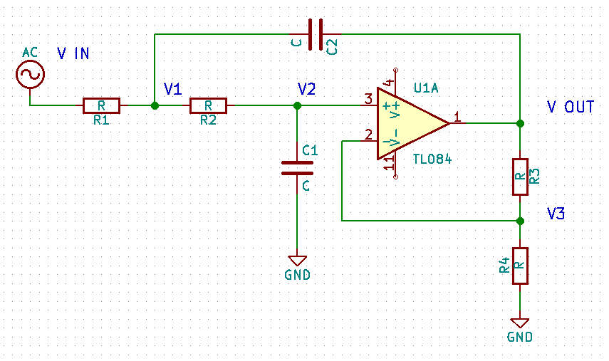

From the field of Electronics and Electrical engineering there are great tools available to analyze the system without much difficulty. The concepts which are used are Nodal Voltage Analysis of circuits, Laplace transformation to convert from the time domain to the frequency domain and a bit of Control Theory to study the system after obtaining the equation.

Deriving the equations

For the case of op amps and active filters a couple of assumptions must be made for the analysis.

• Input Impedance is close to infinity
• Output Impedance is close to zero
• The voltage difference between input terminals (V+ and V-) is zero

We start by converting the capacitors to impedances (Z) in the frequency domain.

Z1= 1 / (s c1);
Z2 = 1/ (s c2);

Establish the equations for each node (V1, V2, V3)

eq01 = (v1 - vin)/R1 + (v1 - v2)/R2 + (v1 - vout)/Z2 == 0;
eq02 = (v2 - v1)/R2 + v2/Z1 == 0;
eq03 = (v3 - vout)/R3 + v3/R4 == 0;

As mentioned earlier, the input voltage difference accross voltage terminals is zero. Thus

v2 = v3;

We now solve the system of equations

{solutionLP} = Solve[{eq01, eq02, eq03}, {v1, v2, vout}]

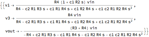
We obtain the transfer function for the system which describes the relation between output and input

H(s) = Voutput / Vinput (* Transfer function equation in control theory*)
LP = vout/vin /. {solutionLP} (* Transfer function for the Low Pass Filter *)

Let us now give values to the capacitors and resistors to simulate its behavior

parameters = {R1 -> 1000, R2 -> 1000, R3 -> 100, R4 -> 100, c1 -> 0.000001, c2 -> 0.000001}

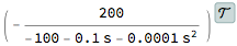
Use the appropriate functions in Mathematica to get a transfer function model

tfLP = TransferFunctionModel[vout/vin /. {solutionLP}, s] /. parameters

Let us now see how the system responds to different input signals and frequencies

out01 = OutputResponse[tfLP, Sin[5000 t], t];
Plot[out01, {t, 0, 1/100}]

out02 = OutputResponse[tfLP, UnitStep[t], t]
Plot[out02, {t, 0, 0.02}, PlotRange -> All]

We can get a more useful visualization by plotting the dB gain of the output depending on the frequency

LogLinearPlot[20 Log[Abs[tfLP[I frequency]]], {frequency, 0, 10000}]

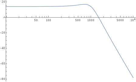
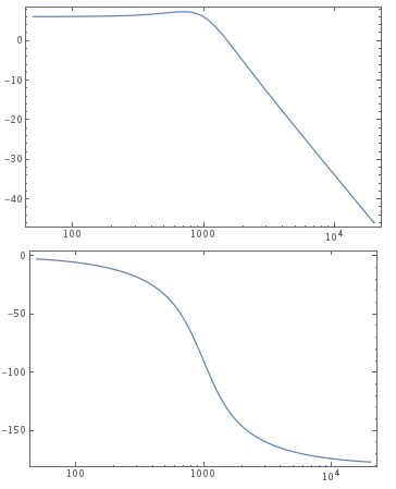
A smarter way to do the same is with a built-in function

BodePlot[tfLP]

Conclusion

Overall, Mathematica proves that what could have taken me about three hours of work by hand can be done in less than ten minutes. This speeds up dramatically the process of learning about a new topic in Electronics and implementing a design for a specific problem. One can easily make several iterations of the system, coupled with other equations to obtain proper values for the passive components of the filters and simulate its response in mere seconds.

To Do

I'd love to expand a bit more on this topic, adding the equations for the others filtered mentioned. Of course more useful examples would be provided from my own notes and real world comparisons. The example shown above was created just for this demonstration and can obviously be improved as well.