A new example has been added to the collection of ready-made example models available on the SystemModeler site: Hare-Lynx: Interactively Explore Population Dynamics. The model requires the free SystemDynamics Modelica library, which can be downloaded from here.

The model uses predator-prey equations, also known as Lotka-Volterra equations. It aims to describe a biological system consisting of two species, a predator (here lynx) and a pray (here hares) and the interaction between them. A large number of predators in the system will increase the mortality of the prey due to predation. A low number of prey will decrease the viability of the predator due to starvation.

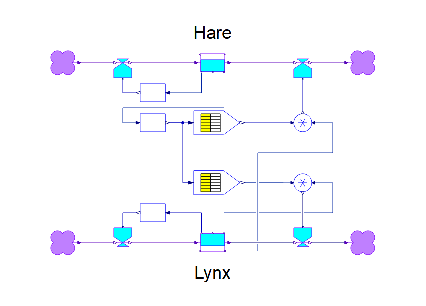
While they can be useful for describing phenomenon in nature, what is very interesting about these systems is their mathematical properties. Solving the system will yield a periodic solution that is something akin to a harmonic motion:

Needs["WSMLink`"]

WSMPlot["HareLynxPopulation", "Population Levels", Ticks -> None]

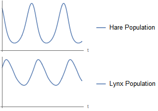
The predator is lagging the population growth of the prey by 90° in the period solution, but otherwise the populations are stable over time.

There are important parameters that affect these equations. The initial conditions are one of them, the rate at which hares and lynx are born is another. If we want to explore these four parameters, we can make use of one of SystemModeler 5s latest features, WSMParametricSimulateValue.

In essence, what it does is it treats a SystemModeler model just as any other Wolfram Language function. You give it a set of arguments and from the function you get the trajectories of some variables over time. It is easy to set up these functions, you just give it the model name, the variables that you want to get back when you call the function, and the parameters that you want to give as arguments:

sim = WSMParametricSimulateValue["HareLynxPopulation", {"hare", "lynx"}, 
    {"HareInitialPopulation", "LynxInitialPopulation", "HareBirthFactor", "LynxBirthFactor"}, 
    WSMProgressMonitor -> False]

Now you can call the function with arbitrary arguments and get back a result:

sim[30000, 2000, 1.25, 0.25]

You can use this directly to plot the two populations:

Map[ListLinePlot, sim[30000, 2000, 1.25, 0.25]]

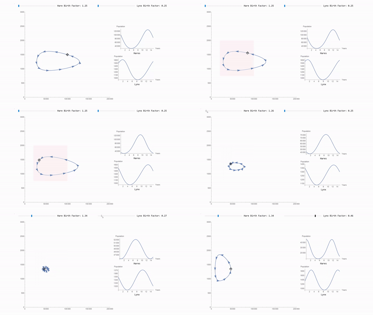
Of even more interest could be to look at a parametric plot of the system, with the population of hares (x-axis) versus the population of lynx (y-axis).

ParametricPlot[
 Evaluate[Through[sim[30000, 2000, 1.25, 0.25][t]]], {t, 0, 15},
 AspectRatio -> 1, PlotRange -> {{0, Automatic}, {0, Automatic}}
 ]

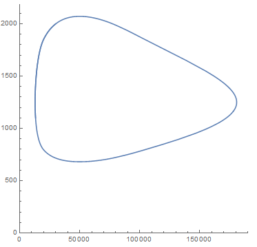
Since it works as any other Wolfram Language function, you can put it inside of a manipulate. For example, here you can explore how the model responds to changing the birth rates for the two species:

Manipulate[
 ParametricPlot[
  Evaluate[Through[sim[30000, 2000, hareBirthFactor, lynxBirthFactor][t]]], {t, 0, 15},
  AspectRatio -> 1, PlotRange -> {{0, Automatic}, {0, Automatic}}
  ],
 {{hareBirthFactor, 1.25}, 1.2, 1.5},
 {{lynxBirthFactor, 0.25}, 0.2, 0.5},
 ContinuousAction -> False
 ]

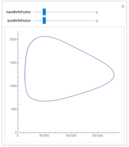
The downloadable example shows how a much more advanced interactive exploration can be constructed in the same vein. Here is a sneak peak of it using a locator pane:

Learn about this and many more new SystemModeler 5 features on the What's New page.

Attachments: