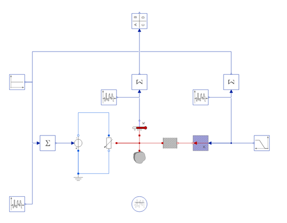
A new example has been added to the collection of ready-made example models available on the SystemModeler site: Evaluating the Robustness of a Temperature State Estimator.

This model analyzes the robustness of a state estimator, taking measurements from an electrical radiator. The state estimator blends together different measurements and a model of the system in order to estimate the current radiator temperature. To evaluate the robustness, noise is added using blocks from the Modelica.Noise library.

The Noise library was of the new libraries added in SystemModeler 5.0 (also see Modelica.Media and Modelica.Electrical.PowerConverters).

In this post, I figured I would dive a bit into how the Noise library works. First, I will load the Wolfram SystemModeler Link:

Needs["WSMLink`"]

The Noise library generates pseudo-random reproducible noise. Reproducibility is key in many control design scenarios. For example, say you are comparing how well two different control systems respond to measurement noises. While you want the noises to be random, at the same time you will want the control systems to experience the same kind of signal outliers at the same time.

Simulating the output from the Modelica.Blocks.Noise.NormalNoise twice will yield identical results. The seed for the random number generator can be manually set, and setting the same seed in two simulations will also yield identical results:

GraphicsGrid[{
  {
   WSMPlot[WSMSimulate["Modelica.Blocks.Noise.NormalNoise", {0, 1}], 
    "y", PlotLabel -> "Seed: Default"], 
   WSMPlot[WSMSimulate["Modelica.Blocks.Noise.NormalNoise", {0, 1}], 
    "y",
    PlotLabel -> "Seed: Default"]
   },
  {
   WSMPlot[
    WSMSimulate["Modelica.Blocks.Noise.NormalNoise", {0, 1}, 
     WSMParameterValues -> {"fixedLocalSeed" -> 42, 
       "useAutomaticLocalSeed" -> False}],
    "y", PlotLabel -> "Seed: 42"],
   WSMPlot[
    WSMSimulate["Modelica.Blocks.Noise.NormalNoise", {0, 1}, 
     WSMParameterValues -> {"fixedLocalSeed" -> 42, 
       "useAutomaticLocalSeed" -> False}],
    "y", PlotLabel -> "Seed: 42"]
   }
  }, ImageSize -> Large, Frame -> {False, True}]

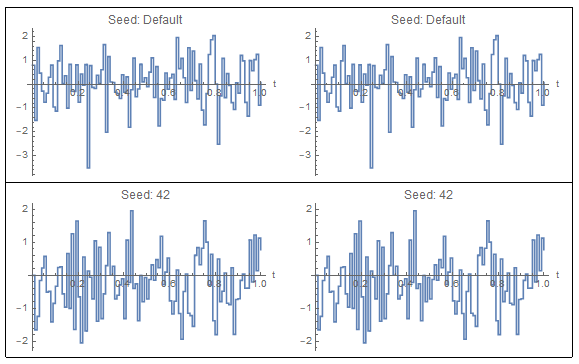
As you can see, the generated noise is discrete samples drawn from a distribution at fixed sampling points.

Using the new RawData property of WSMSimulationData, we can create a Histogram of the noisy observations. The "mu" and "sigma" parameters are the mean and standard deviation for the normal distribution.

Histogram[
 WSMSimulate["Modelica.Blocks.Noise.NormalNoise", 
    WSMParameterValues -> {"mu" -> 1, "sigma" -> 0.1, 
      "samplePeriod" -> 0.05}]["RawData", "y"][[All, 2]]]

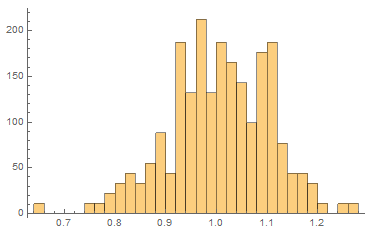
With the Probability & Statistics functionality in the Wolfram Language, we can get the probability density function for the same distribution.

PDF[NormalDistribution[1, 0.1], x]

3.98942 E^(-50. (-1 + x)^2)

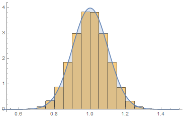
We can also overlay the PDF on the histogram.

Show[Histogram[
  WSMSimulate["Modelica.Blocks.Noise.NormalNoise", 
     WSMParameterValues -> {"mu" -> 1, "sigma" -> 0.1, 
       "samplePeriod" -> 0.05}]["RawData", "y"][[All, 2]],
  Automatic, "PDF"],
 Plot[PDF[NormalDistribution[1, 0.1], x], {x, 0.5, 1.5}, 
  Filling -> Axis]
 ]

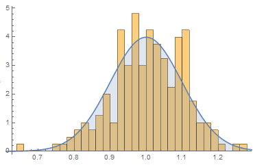
As the number of observations tend to infinity, the observations will fit the distribution better and better. We can simulate this by either increasing the simulation time or (as seen below) by decreasing the sample period.

In the downloadable example a Kalman filter estimator was created by linearizing the model without noise, using the function WSMLinearize. The filter can then be used to estimate the true state of a system, even when it is subjected to heavy noise. The construction of such a filter is a bit outside the scope of this post, but if there is interest, I can make a separate post with the linear time-invariant capabilities of the Wolfram Language and SystemModeler. For now, you can download this model and try out the Noise library that is included in SystemModeler 5.0 from here.

Attachments: