This demonstration is about how to numerically solve a classic mechanical problem and visualize the result. Given a conic cantiliver beam with its large end plugged into a solid wall. Its cross-sections are circles. The length of the beam is 0.3 m and the diameter follows:
d[x_] := 0.0635 - (0.0635/2)*x/length
where the thick end is at x = 0 and the thin end is at x = 0.3. If I assume the material is aluminium and then I can find the shear modulus using wolfram alpha:
In[1]:= Cases[
WolframAlpha["aluminium", {{"Material:ElementData", 1}, "ComputableData"}, PodStates -> {"Material:ElementData__More"}],
{"shear modulus", _}]
Out[1]= {{"shear modulus", Quantity[26, "Gigapascals"]}}
We also know the second moment of inertia of this beam is
polarMoment[x_] := (\[Pi]*d[x]^4)/32;
Now lets add a 10 Nm torque at the thin end of this beam, we can solve the deformation by finite difference method here, which is embedded in the NDSolve function with simple boundary condition:
length = 0.3;
shearModulus = 26*10^9;
torque = 10;
sol = NDSolve[{D[shearModulus*polarMoment[x]*D[\[Theta][x], x], x] == -torque, \[Theta][0] == 0, \[Theta]'[0] == torque/(
polarMoment[0]*shearModulus)}, \[Theta], {x, 0, length}]
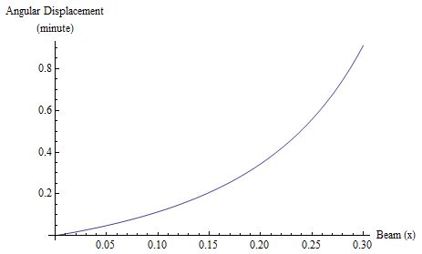
The plot is
Plot[Evaluate[\[Theta][x] /. sol[[1]]]/\[Pi]*180*60, {x, 0, length},
AxesLabel -> {"Beam (x)", "Angular Displacement\n(minute)"},
LabelStyle -> 12
]
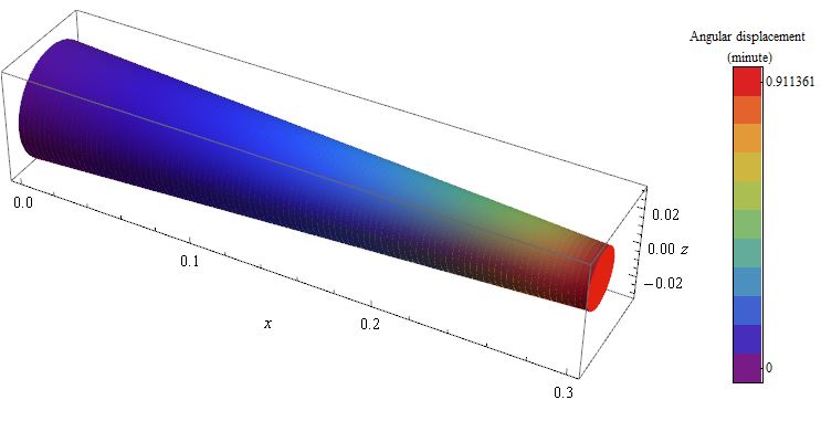
To make a thermograh for this beam, we can simply stack a list of cylinders with variable diameter and apply a piece of color base on the which scale it is on (of course the better way would be using GraphicsComplex and Polygon) . The scale can be automatically specified with the range of the numerical solution and Rescale can convert the range to proper color scale:
min = 0;
max = NMaximize[{Evaluate[\[Theta][x] /. sol[[1]]], 0 <= x < length}, x][[1]]/\[Pi]*180*60
Now we can create a pseudo conic shape (dx is the thickness of each slice):
dx = length/100;
cylinders = Table[
{
EdgeForm[],
ColorData["Rainbow"][
Rescale[Abs[
Evaluate[\[Theta][i] /. sol[[1]]]]/\[Pi]*180*60, {min,
max}]], Cylinder[{{i, 0, 0}, {i + dx, 0, 0}}, d[i]/2]
},
{i, 0, length - dx, dx}];
Graphics3D can handle a list of graphics objects easily. I used a ArrayPlot to create a color bar, which is slightly tricky.
Row[{
Graphics3D[cylinders, Axes -> {True, False, True},
AxesLabel -> {x, None, z}, LabelStyle -> Directive[FontSize -> 15]],
ArrayPlot[Table[{1 - i}, {i, 0, 1, 0.1}],
ColorFunction -> "Rainbow",
PlotLabel -> "Angular displacement\n (minute)",
FrameTicks -> {{None, {{11, min}, {1, max}}}, {None, None}},
FrameTicksStyle -> 12]}
]
The result is surprisingly "professional":