Introduction
Elections are fundamental to our democracies and way of life. The electorate bestows power on the lawmakers and public officials whose legitimisation is derived solely from the fact that they are elected. In recent times, many elections, such as the presidential elections the United States and the Brexit and general elections in the United Kingdom have seen a very pronounced polarisation the electorate. Can mathematics and the Wolfram Language help to better understand this crucial process of the most fundamental decision making process in societies? The main question I want to discuss in a sequence of posts is what can be learnt from elections. So this post is about computational politics.
It is important to notice that democracies rely on a general acceptance of the result of elections. Without that consensus a peaceful co-existence is at risk. Societies agree on certain electoral procedures and the results have to be understood to be final. There are, however, more fundamental questions such as how do we derive the "voters will" from ballots. That is a highly non-trivial problem. Also, elected politicians often claim that they represent the "will of the people". But is that true and what is the "will of the people"? Hence, my question: the voters have spoken - but what did they say?
This is the third of a series of posts:
- Electoral systems - interpreting the will of the voters
- Gerrymandering - shaping the voters' will to your liking
- Analysis of the Brexit vote - how do we know what did the voters really want?
This part of the sequence of posts will analyse the results of the Brexit vote in the United Kingdom. The question asked was basically a yes/no question and with small majority the social choice was to conduct Brexit. The rules of this process have been followed and the decision is binding. There is, however, a related question: Did the outcome in this particular case actually give sufficient evidence that this is the "will of the people" as many politicians state. If we want to evaluate the power of evidence there are mathematically established procedures. Similar procedures are for example applied in medical trials to evaluate the evidence provided by data to support a particular hypothesis. We will apply this type of procedure to the Brexit elections.
All posts were developed with Bjoern Schelter, who is also a member of this community. He is indeed the expert on these methods.
Disclaimer: this post might be modified slightly over the next couple of days.
Data download and preparation
We will start by obtaining some of the data required for this post. The central dataset is provided by the electoral commission. It is attached to this post. We download and them import the data like so:
SetDirectory[NotebookDirectory[]]
votingData = Import["EU-referendum-result-data.csv"];
Here is a short extract of the data:
votingData[[1 ;; 5]] // Transpose // TableForm
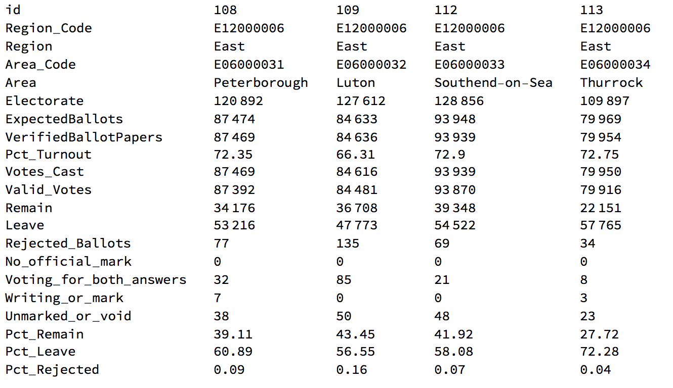
Next, we will need some data on the local authorities/electoral districts from here. We then import:
localauthorities = Import["Local_Authority_Districts_December_2016_Generalised_Clipped_Boundaries_in_Great_Britain.shp"];
explanationShape = Import["Local_Authority_Districts_December_2016_Full_Clipped_Boundaries_in_Great_Britain.csv"];
These data sets contain information about the shape and location of the local authority boundaries and data on how to match that with the voting outcome in the first file. To get a first glance at the data we re-arrange and organise the data like so:
Monitor[areas =
   Table[QuantityMagnitude[UnitConvert[If[Length[#] > 1, Total[GeoArea /@ #], GeoArea[#]]], "SI"] & @(localauthorities[[1, 2, 1, 2, 1, 2, 1, 1, 1]][[k]]), {k,         1, Length[localauthorities[[1, 2, 1, 2, 1, 2, 1, 1, 1]]]}];, k]
and
translateshpvote = SortBy[(Flatten /@ Transpose[{SortBy[Transpose[{Range[380], areas}], Last], SortBy[explanationShape[[2 ;;]], #[[9]] &]}])[[All, {1, 4}]], First];
The first representation is not very telling. It shows the outcome of the election.
Graphics[Flatten[
  Table[{ColorDataFunction["TemperatureMap", "Gradients", {0, 1}, Blend["TemperatureMap", #]& ][(Select[
  votingData[[2 ;;]], #[[4]] == translateshpvote[[k, 2]] &][[1]])[[-3]]/100.], localauthorities[[1, 2, 1, 2, 1, 2, 1, 1, 1]][[k]]}, {k, 1, 380}],1], AspectRatio -> GoldenRatio]
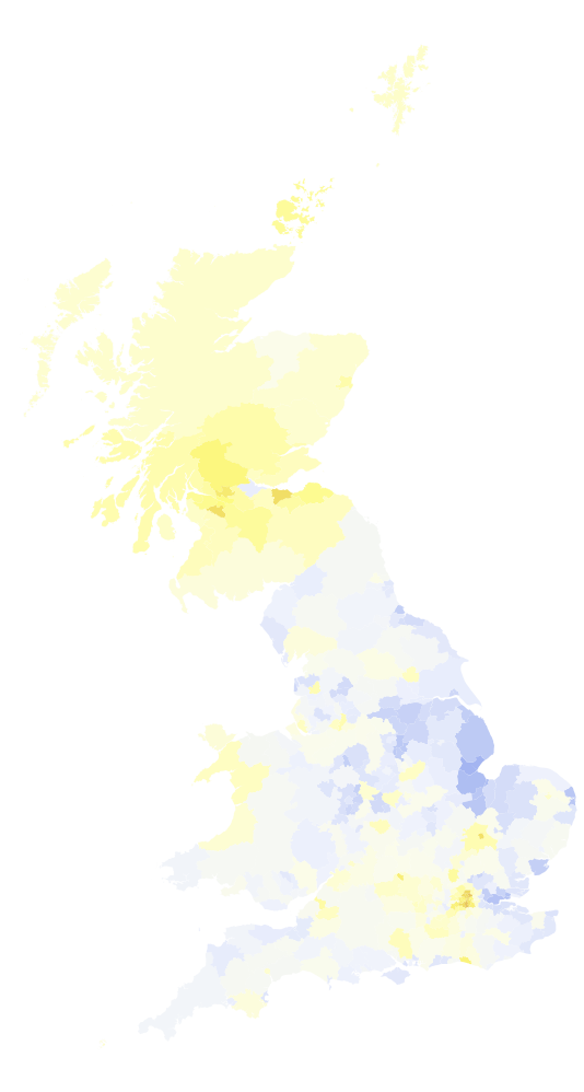
The "blue-r" the colour the higher the percentage of leave votes. Yellow indicates a preference for remain. We will need to clean the data further and will then plot it with a threshold to see which regions decided for Leave and which ones for Remain:
substitute = ({#[[1]][[{1, 4}]] -> #[[2]][[{1, 4}]], #[[2]][[{1,
4}]] -> #[[1]][[{1, 4}]]} &@((Flatten /@
Transpose[{SortBy[Transpose[{Range[380], areas}], Last],
SortBy[explanationShape[[2 ;;]], #[[9]] &]}])[[205 ;; 206]]))

translateshpvoteclean = translateshpvote /. substitute;

Graphics[Flatten[
Table[{ColorDataFunction["TemperatureMap", "Gradients", {0, 1}, Blend["TemperatureMap", #]& ][
If[# > 0.5, 1, 0] & @((Select[Select[votingData[[2 ;;]], #[[1]] < 381 &], #[[4]] == translateshpvoteclean[[k, 2]] &][[1]])[[-3]]/100.)],
localauthorities[[1, 2, 1, 2, 1, 2, 1, 1, 1]][[k]]}, {k, 1, 380}],1], AspectRatio -> GoldenRatio]
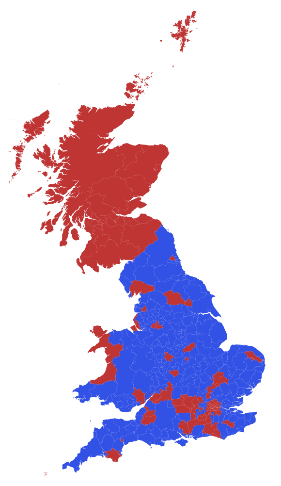
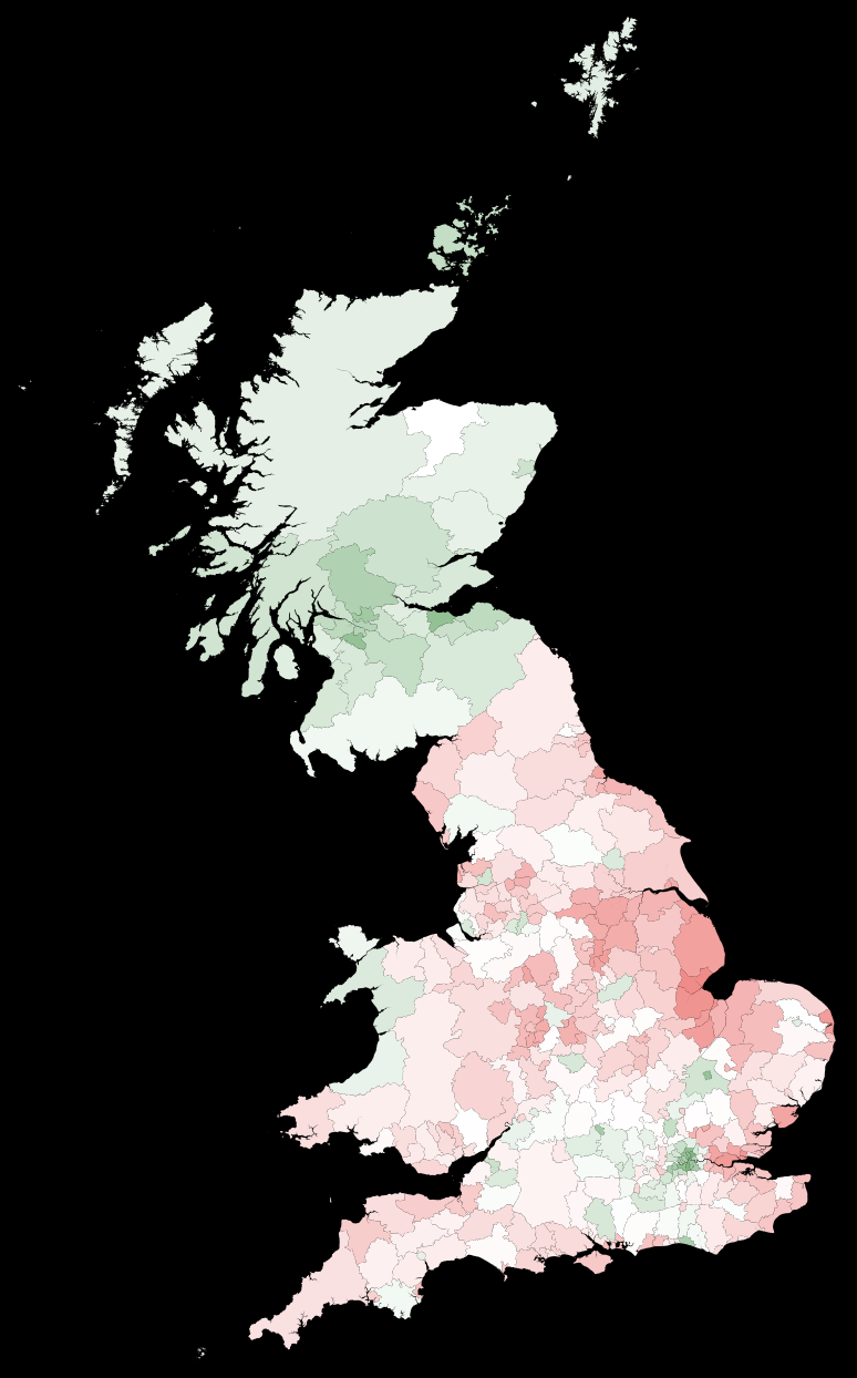
The strong divide between England and Scotland becomes apparent from that figure. We will use the following style of the image in much of the remainder of the post:
Graphics[Flatten[
  Table[{ColorData[
      "RedGreenSplit"][((Select[
           Select[votingData[[2 ;;]], #[[1]] < 381 &], #[[4]] ==
             translateshpvoteclean[[k, 2]] &][[1]])[[-3]]/100.)],
    localauthorities[[1, 2, 1, 2, 1, 2, 1, 1, 1]][[k]]}, {k, 1, 380}],
   1], Background -> Black, AspectRatio -> GoldenRatio]
What does the Brexit election outcome tell us? What did voters want?
UK wide the percentage of leave votes (with respect to all valid votes) is:
N[Total[votingData[[2 ;;, 13]]]/Total[votingData[[2 ;;, 11]]]]
51.89%. This is in percentage of all valid votes. The percentage of leave with respect to the entire electorate is:
N[Total[votingData[[2 ;;, 13]]]/Total[votingData[[2 ;;, 6]]]]
37.4%. This is the percentage of the entire electorate who voted for remain.
N[Total[votingData[[2 ;;, 12]]]/Total[votingData[[2 ;;, 6]]]]
34.7%. The percentage of non-voters is:
N[(Total[votingData[[2 ;;, 6]]] - Total[Flatten@votingData[[2 ;;, 12 ;; 13]]])/Total[votingData[[2 ;;, 6]]]]
27.8%. This means that we do not know the will of about 28% of all voters. Following the predefined social choice procedure, the vote was narrowly won by leave. That does not necessarily imply that this is "the will of the majority of people".
What would the result be with indirect representation?
If we had a representational vote we would have to count the districts for remain and leave
{Count[#, "Remain"], Count[#, "Leave"]} &@((#1 > #2) & @@@ votingData[[2 ;;, {12, 13}]] //. {False -> "Leave", True -> "Remain"})
{119,263}. This result is even more extreme for leave. This is because the population in the local authorities is very different.
Histogram[votingData[[2 ;;, 6]], PlotRange -> All, PlotTheme -> "Marketing", ImageSize -> Large,
FrameLabel -> {"population", "number of authorities"}, LabelStyle -> Directive[Bold, 15]]
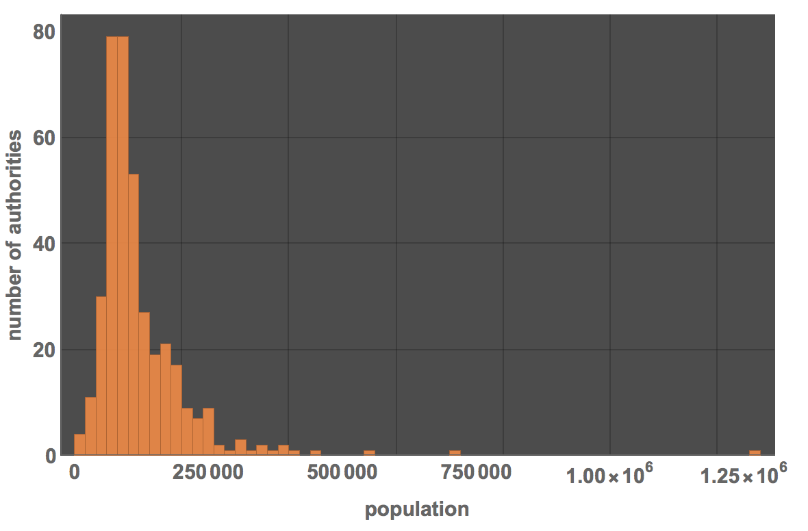
This shows that there are large fluctuations in the population of the areas. Let's represent that slightly differently. We first collect data about Leave votes, Electorate, Turnout and Electorate.
electionEUresolved =
  Transpose@({#[[1]], #[[2]], #[[3]], #[[4]]} &@Transpose@((({#[[13]], #[[11]], #[[9]], #[[6]]} & /@ (Reverse@SortBy[votingData[[2 ;;]], #[[9]] &])))));

BubbleChart[{#[[3]], N@#[[1]]/#[[2]], #[[4]]} & /@ electionEUresolved,
  BubbleSizes -> Small,
 ChartLabels ->
  Placed[(Reverse@SortBy[votingData[[2 ;;]], #[[9]] &])[[
    All, {5, 3}]], Tooltip],
 Epilog -> {Red, Line[{{50, 0.5}, {100, 0.5}}]},
 PlotTheme -> "Marketing", BubbleScale -> "Area", ImageSize -> Large,
 FrameLabel -> {"turnout", "percentage leave votes"},
 LabelStyle -> Directive[Bold, 15]]
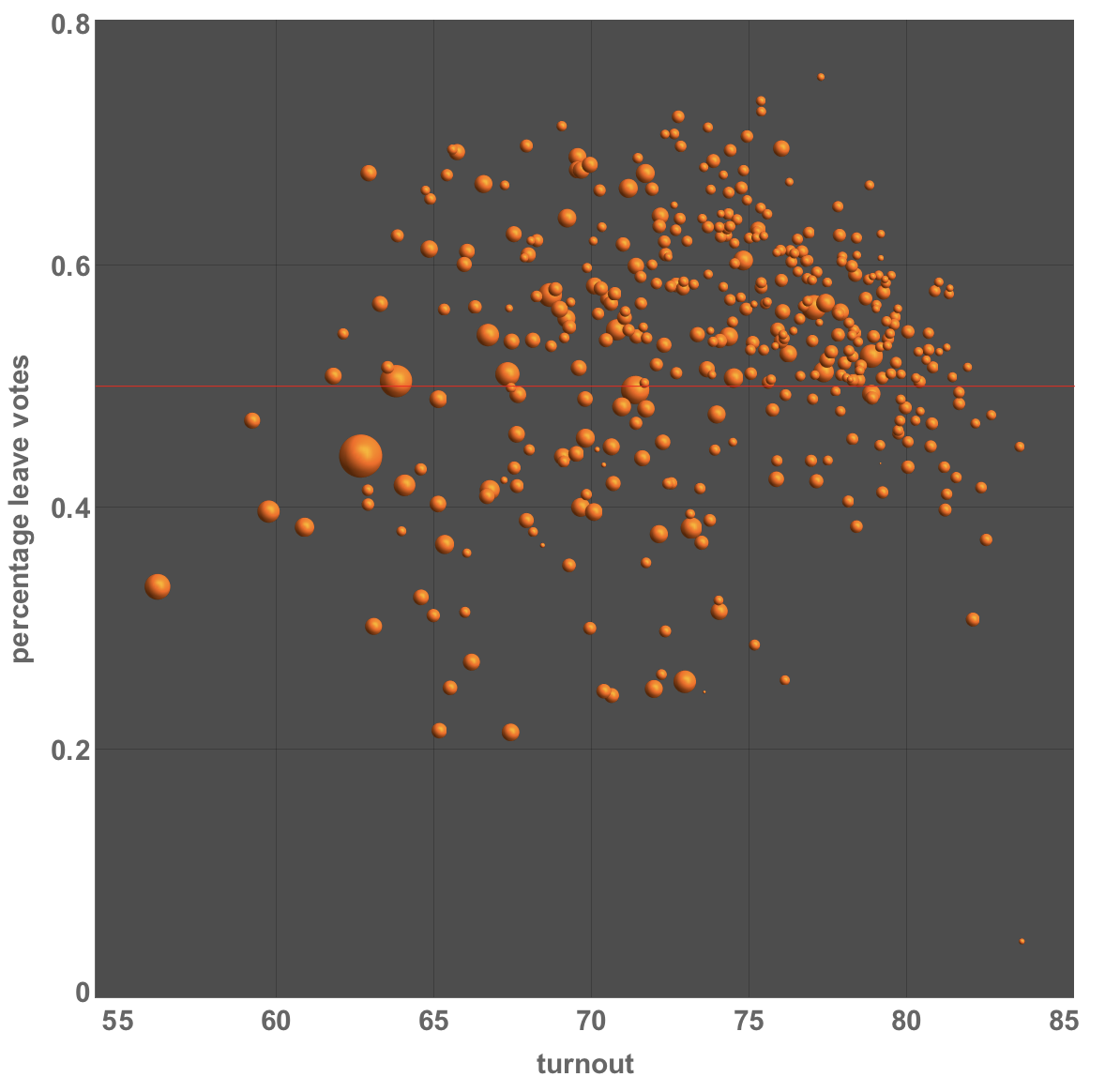
The bubble sizes (areas) correspond to the size of the electorate. Let's see whether there is a correlation with turnout:
lm = LinearModelFit[{#[[3]], N@#[[1]]/#[[2]]} & /@ electionEUresolved,x, x, Weights -> electionEUresolved[[All, 4]]]

The following table shows that the positive slope is highly significant.
lm["ParameterTable"]

We can add that to the figure:
Show[BubbleChart[{#[[3]], N@#[[1]]/#[[2]], #[[4]]} & /@
   electionEUresolved, BubbleSizes -> Small,
  ChartLabels ->
   Placed[(Reverse@SortBy[votingData[[2 ;;]], #[[9]] &])[[
     All, {5, 3}]], Tooltip],
  Epilog -> {Red, Line[{{50, 0.5}, {100, 0.5}}]},
  PlotTheme -> "Marketing", BubbleScale -> "Area", ImageSize -> Large,
   FrameLabel -> {"turnout", "percentage leave votes"},
  LabelStyle -> Directive[Bold, 15]],
 Plot[lm[x], {x, 50, 85}, PlotStyle -> White]]
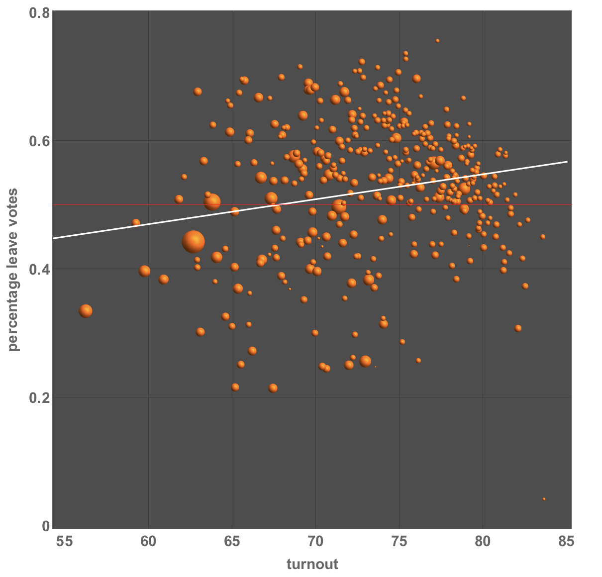
Seeing such a linear dependence, raises the natural question to which extent the result is biased by such correlations in the data. Linear Models are a powerful tool to account for various potential influencing factors on the final outcome of the election.
Linear Modelling
Linear Models are a generalisation of linear regression; linear models allow us to model a Gaussian Distributed outcome by various inputs that may or may not be continuous. To demonstrate this we use the simple voting data; the dependent, outcome, variable is the percentage of people who voted to leave the EU.
percentleave = N[votingData[[2 ;;, 13]]/votingData[[2 ;;, 11]]];

collatedData = (Flatten /@
    Transpose[{Table[
       Select[votingData, explanationShape[[k, 2]] === #[[4]] &], {k,
        2, Length[explanationShape[[1 ;;]]]}],
      explanationShape[[2 ;;]]}]);
We can then prepare the data for the linear model:
inputLinearModel =
Flatten /@ Transpose[{# - Mean[#] &@ collatedData[[All, 9]], collatedData[[All, 3]], # - Mean[#] &@ (collatedData[[All, 6]]/collatedData[[All, 30]]),
N[collatedData[[All, 13]]/collatedData[[All, 11]]]}];
The steps above generate the table that defines the input into the linear model. All continuous input variables have been centralised such that their mean is zero. This is not needed but simplifies the interpretability of the results. This input variables to the linear model are turnout, i.e., the fraction of people who voted in the given local administrative area, region, i.e., the rough geographical region (non continuous, nominal variable), and a proxy for the population density.
lmodel = LinearModelFit[inputLinearModel, {turnout, region, popdensity}, {turnout, region, popdensity}, NominalVariables -> region];
lmodel["ParameterTable"]
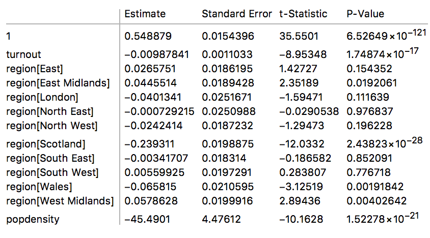
The model output shows the estimates with respect to the intercept (1) in the table. The missing region is Yorkshire and The Humber such that Mathematica relates all results to this region. Note, that the estimate of 0.548879 means that Yorkshire and The Humber would have voted to leave the EU with 54.89%; this is the model output and does not necessarily match the actual result of the election. Since all continuous variables are mean zero, these 54.89% would be the result for Yorkshire and The Humber under the assumption that the have a typical UK average population density and turnout. The model can obviously be used to approximate the result for Yorkshire and The Humber better by evaluating the function with the correct values for the area. All other influencing factors are estimated with respect to this result. In other words to obtain the result for Scotland, the Scotland result would need to be added to the Yorkshire and The Humber result; so the best model guess for Scotland if otherwise indistinguishable from the while UK would have been -23.93%+54.89%=30.96%. This obviously deviates from the actual result for Scotland, which is likely caused by the other covariates, the turnout and population density in Scotland are different from the average UK value.
Next we want to analyse the same model but with data for Gibraltar and Ni added. We first need the respective areas of the regions:
fixNIGI =
  Join[#[[1 ;; -2]],
     ConstantArray[Missing[],
      8], {#[[-1]]}, {Missing[]}] & /@ (Flatten /@
     Transpose[{Select[
        votingData, #[[1]] > 380 &], {QuantityMagnitude[
         UnitConvert[
          Entity["AdministrativeDivision", {"NorthernIreland",
             "UnitedKingdom"}]["Area"], Quantity[1, (("Meters")^2)]]],
         QuantityMagnitude[
         UnitConvert[Entity["Country", "Gibraltar"]["Area"],
          Quantity[1, (("Meters")^2)]]]}}]);
Then we can add the data to the table, create the input the linear model and estimate it:
collatedDatacomplete = Join[collatedData, fixNIGI];

inputLinearModelcomplete =
Flatten /@ Transpose[{# - Mean[#] &@ collatedDatacomplete[[All, 9]],
collatedDatacomplete[[All, 3]], # - Mean[#] &@ (collatedDatacomplete[[All, 6]]/collatedDatacomplete[[All, 30]]),
N[collatedDatacomplete[[All, 13]]/collatedDatacomplete[[All, 11]]]}];

lmodelcomplete = LinearModelFit[inputLinearModelcomplete, {turnout, region, popdensity}, {turnout, region, popdensity}, NominalVariables -> region]

lmodelcomplete["ParameterTable"]
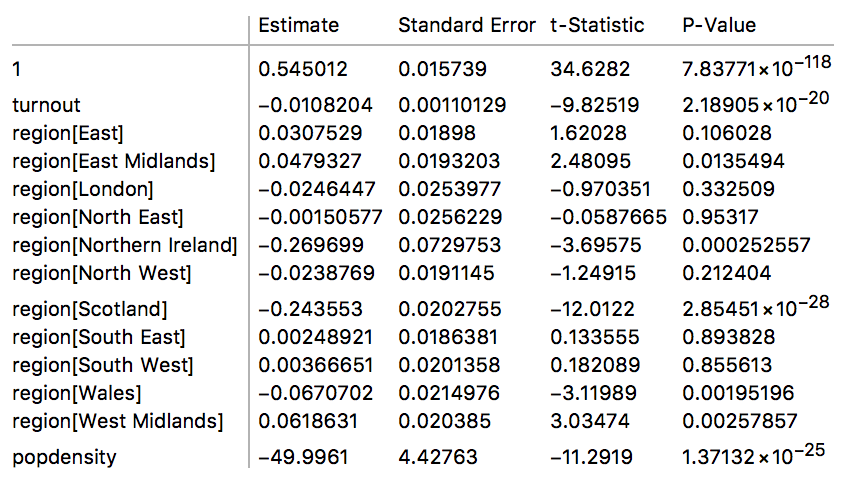
The values match the result above quite well, obviously there is now a result for NI as well. The key thing about linear models is that one can combine the various areas to get a area weighted estimate for the election result. To achieve this we need to obtain the parameters from the table above.
parametermatrix = Delete[lmodelcomplete["ParameterTableEntries"], {{2}, {-1}}]
To achieve a area weighted result, we need to obtain the weights for each region which is defined as the number of entries per area divided by the total number of entries:
weights = N[#/Total[#]] &@RotateRight[SortBy[Tally[inputLinearModelcomplete[[All, 2]]], First]][[All, 2]]
As all parameters are given with respect to one area and present differences to this area, we need to add all estimates to the intercept, see example for Scotland above. This is achieved through linear algebra, by defining a so called contrast matrix.
contrast = IdentityMatrix[Length[weights]];
contrast[[1]] = ConstantArray[1, Length[weights]];
contrast = Transpose[contrast]
Multiplying the matrix to the parameter estimates gives the response functions, the model results for each area.
responsefunctions = contrast.parametermatrix[[All, 1]]
Multiplying this with the weights for each area results in a weighted mean for the UK. It is worth noting that this result is no longer influenced by the turnout and the average population density as these are 0 for the UK, as we subtracted their overall mean in the beginning.
weights.responsefunctions
So the model's referendum result would have been 52.99% in favour of leave, so higher than the actual result. Importantly, Linear Models provide errors for each parameter estimate, such that we can estimate the overall uncertainty of this result. As standard errors are not additive but variances are, we obtain the estimated standard error for this result as follows, assuming independence of the estimates
seresponsefunctions = contrast.(parametermatrix[[All, 2]]^2)
The final standard error is
Sqrt[weights.seresponsefunctions]
0.0255668. This means that best model guess is that 52.99% p/m 2.56% are in favour of leave, using a Gaussian approximation, this implies that there is a
Probability[x < -(weights.responsefunctions - 0.5)/Sqrt[weights.seresponsefunctions], x \[Distributed] NormalDistribution[0, 1]]
12.11% chance that this result was obtained although the majority of the UK electorate does actually not want to leave the EU. We emphasise that by no means are we challenging the result of the referendum, we are just arguing that given model assumptions the results obtained are actually compatible with a population split in which the majority does not want to leave the EU. In many fields such as Science and Medicine, a 12.11% 'risk' that the result is actually a false positive, i.e., the conclusions drawn and actions taken are wrong, is considered too high, 5% or 1% are typical values, in particle Physics the threshold is much lower. So it remains to be investigated if statements that the election results reflect the true opinion of the population. Again, we do not challenge the outcome of the election as there are clear rules to the election that are known in advance such as that it is everybody's free choice to vote or not and how the final result is obtained. There is just a potential non-causal link to people's real opinions, which is often assumed but not necessarily correctly so.
Getting more data...
An interesting thing to check is whether we can learn something from adding additional data on the various voting districts. The data is from here. We import the file with the data
additionaldata = Import["EU-referendum-results-and-characteristics-data.xlsx"];
We also use the electoral region id data from above:
ids = collatedDatacomplete[[All, 4]];
Then we need to deal with incomplete data/clean the data up:
fillers = ConstantArray[Missing[], #] & /@ Length /@ additionaldata[[2 ;; 11, 4]];
We now can generate a fixed data table:
fulldatatable =
  Table[Join[collatedDatacomplete[[k]], Flatten@Table[If[Length[#] > 0, #, fillers[[i - 1]]] &@
  Select[additionaldata[[i]], MemberQ[#, ids[[k]]] &], {i, 2, 11}]] /. "" -> Missing[], {k, 1, Length[ids]}];
To better work with the data we then generate a look-up table for the various columns:
datadescriptors =
 Rule @@@ (Transpose[{Range[Length[#]], #}] & @
    Join[votingData[[1]], explanationShape[[1]],
     additionaldata[[2, 9]], additionaldata[[3, 1]],
     additionaldata[[4, 8]], additionaldata[[5, 9]],
     additionaldata[[6, 8]], additionaldata[[7, 4]],
     additionaldata[[8, 8]], additionaldata[[9, 4]],
     additionaldata[[10, 3]], additionaldata[[11, 3]]])
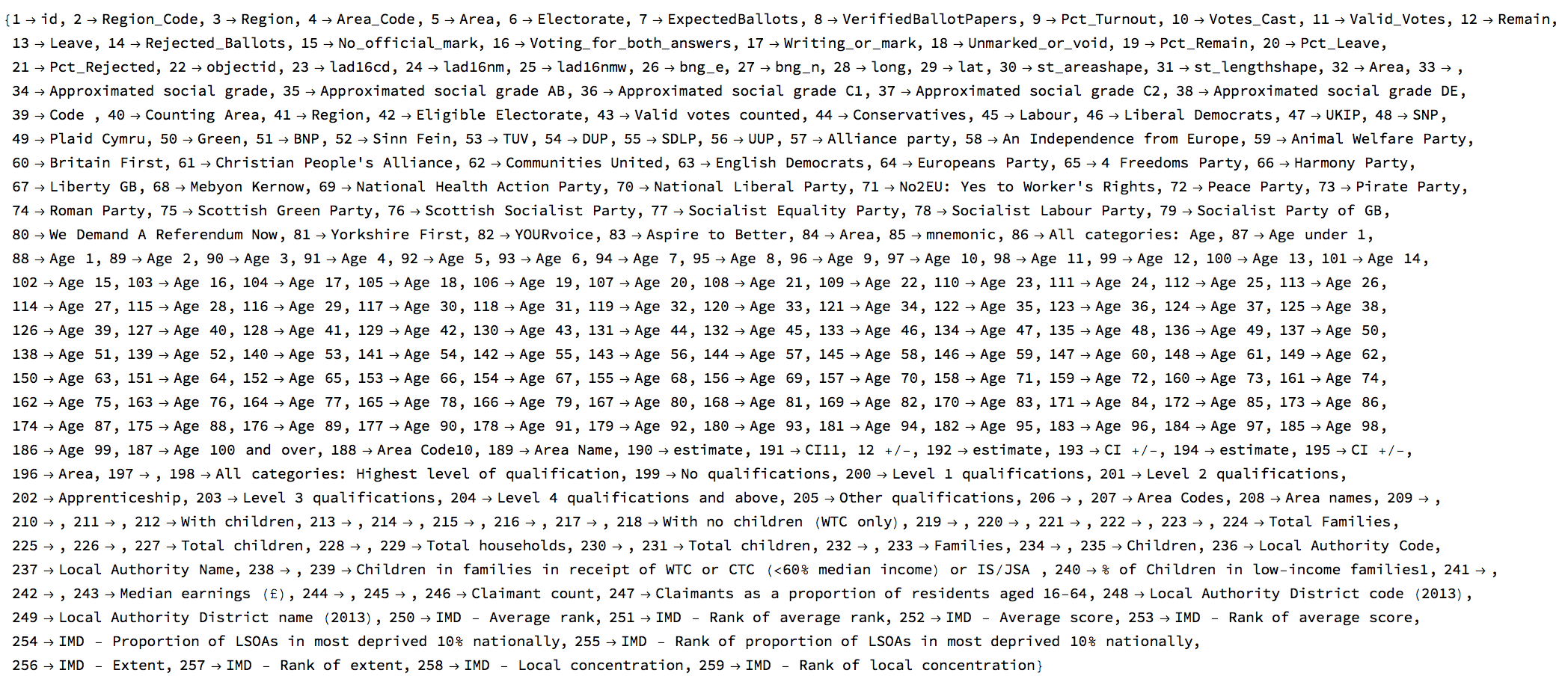
The following shows again a part of the table of all the data we can use now:
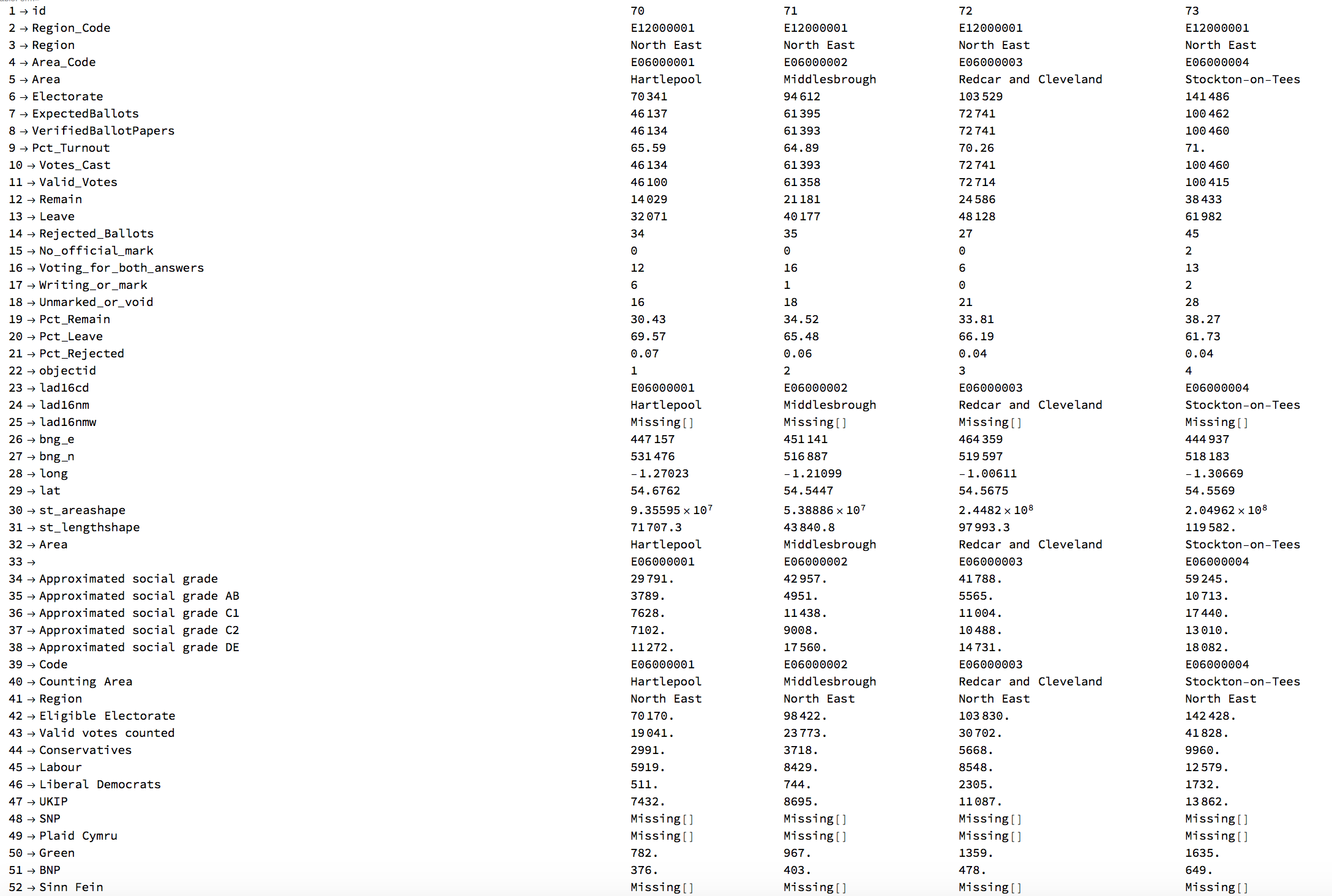
We can then generate some first part of the input for the linear model.
inputLinearModel =
  Flatten /@ Transpose[{# - Mean[#] &@ collatedData[[All, 9]], collatedData[[All, 3]], # - Mean[#] &@ (collatedData[[All, 6]]/collatedData[[All, 30]]),
  N[collatedData[[All, 13]]/collatedData[[All, 11]]]}];
Again we need to clean the data
fulldatatable[[All, 198]] /. "#" -> Missing[]

subMissing[x_] := If[StringContainsQ[ToString[FullForm[x]], "Missing"], Missing[], x ]

SetAttributes[subMissing, Listable]
This generates the full input for the linear model:
inputLinearModelcomplete =
  Flatten /@
   Transpose[{fulldatatable[[All, 3]], (# - Mean[#]) &@
      fulldatatable[[All,
       9]], (# - Mean[#]) &@ (fulldatatable[[All, 6]]/
        fulldatatable[[All, 30]]), (# -
         Mean[DeleteMissing[#]]) &@ (subMissing /@ (fulldatatable[[
           All, 198]]/fulldatatable[[All, 6]])), (# -
         Mean[DeleteMissing[#]]) &@ (fulldatatable[[All, 243]] /.
        "#" -> Missing[]), (# -
         Mean[DeleteMissing[#]]) &@ (subMissing /@ (fulldatatable[[
           All, 227]]/fulldatatable[[All, 6]])),
     N[fulldatatable[[All, 13]]/fulldatatable[[All, 11]]]}];
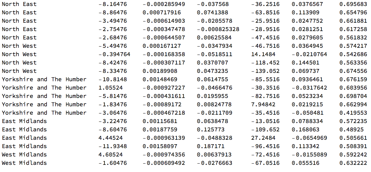
Here are a couple of lines of the input data we choose for our linear model:
inputLinearModelcomplete[[1 ;; 20]] // TableForm
Some more cleaning:
inputLinearModelcomplete = Select[subMissing /@ inputLinearModelcomplete, ! MemberQ[#, Missing[]] &];
Next we fit the linear model:
lmodelfulldata =
  LinearModelFit[inputLinearModelcomplete, {region, turnout, popdensity, highqual, earning, nchildren}, {region, turnout, popdensity, highqual,
  earning, nchildren}, NominalVariables -> {region}];

lmodelfulldata["ParameterTable"]
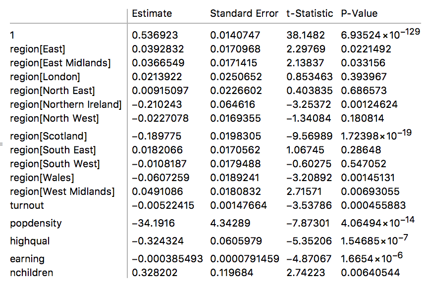
It is easy to see that the income and the number of children in the household significantly influence the preference for/against Brexit. We now use the parameter matrix to compute the weights and contrasts as before:
parametermatrix = lmodelfulldata["ParameterTableEntries"][[1 ;; 12]];
weights = N[#/Total[#]] &@RotateRight[SortBy[Tally[inputLinearModelcomplete[[All, 2]]], First]][[All, 2]];
contrast = IdentityMatrix[Length[weights]];
contrast[[1]] = ConstantArray[1, Length[weights]]; contrast = Transpose[contrast];
With the contrasts we can calculate the response functions:
responsefunctions = contrast[[1 ;; 12, 1 ;; 12]].parametermatrix[[1 ;; 12, 1]]
What is the best estimate for the "will of the voters"?
We an now also use the linear model to estimate what the most likely scenario (based on the model) for the "underlying will of the voter" is given the data from above and the result of the election. We first prepare the data we need, which this time includes the outcome of the election.
inputLinearModelcompletewRcode =
  Flatten /@
   Transpose[{fulldatatable[[All, 4]],
     fulldatatable[[All, 3]], (# - Mean[#]) &@
      fulldatatable[[All,
       9]], (# - Mean[#]) &@ (fulldatatable[[All, 6]]/
        fulldatatable[[All, 30]]), (# -
         Mean[DeleteMissing[#]]) &@ (subMissing /@ (fulldatatable[[
           All, 198]]/fulldatatable[[All, 6]])), (# -
         Mean[DeleteMissing[#]]) &@ (fulldatatable[[All, 243]] /.
        "#" -> Missing[]), (# -
         Mean[DeleteMissing[#]]) &@ (subMissing /@ (fulldatatable[[
           All, 227]]/fulldatatable[[All, 6]])),
     N[fulldatatable[[All, 13]]/fulldatatable[[All, 11]]]}];
This is how the data looks:
inputLinearModelcompletewRcode[[1 ;; 20]] // TableForm
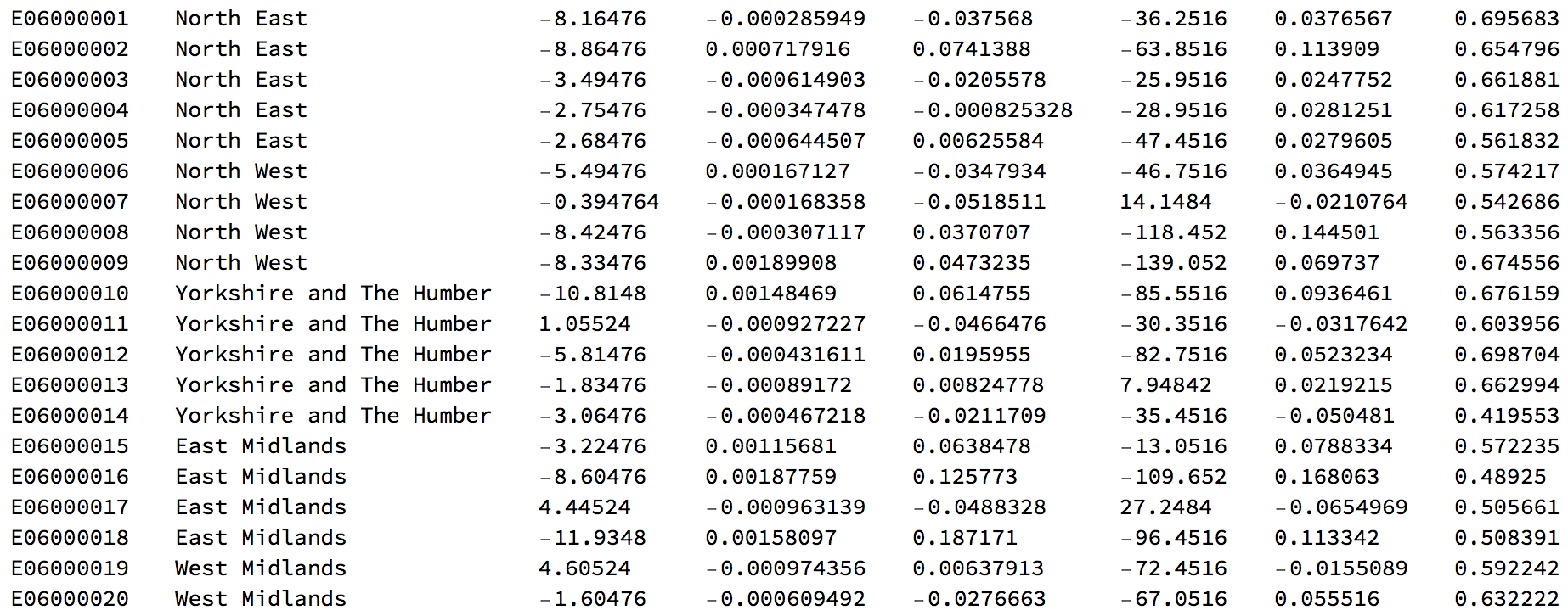
Again we clean the data a bit:
inputLinearModelcompletewRcode = Select[subMissing /@ inputLinearModelcompletewRcode, ! MemberQ[#, Missing[]] &];
Now we can use the linear model to estimate the actual percentage of yes/no votes in the different voting areas:
codepercent = Transpose[{inputLinearModelcompletewRcode[[All, 1]], MapThread[lmodelfulldata, Transpose[inputLinearModelcompletewRcode[[All, 2 ;; -2]]]]}]
First we represent the actual election outcome. Green corresponds to "Remain" and red to "Leave" votes.
Graphics[Flatten[
  Table[{ColorData[
      "RedGreenSplit"][((Select[
           Select[votingData[[2 ;;]], #[[1]] < 381 &], #[[4]] ==
             translateshpvoteclean[[k, 2]] &][[1]])[[-3]]/100.)],
    localauthorities[[1, 2, 1, 2, 1, 2, 1, 1, 1]][[k]]}, {k, 1, 380}],
   1], Background -> Black, AspectRatio -> GoldenRatio]
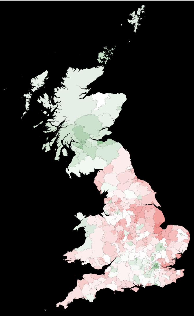
We can now calculate the best estimate of the Leave/Remain split based on our model:
polygonscoloured =
  Table[{ColorData["RedGreenSplit"][1. - ((Select[codepercent, #[[1]] == translateshpvoteclean[[k, 2]] &][[1]])[[-1]]) /. Missing[] -> 0.],
   localauthorities[[1, 2, 1, 2, 1, 2, 1, 1, 1]][[k]]}, {k, 1, Length[translateshpvote]}];

Graphics[polygonscoloured, AspectRatio -> GoldenRatio, Background -> Black]
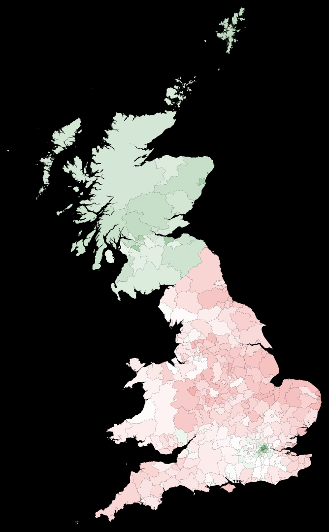
The split between England and Scotland has become even more pronounced. Note that we haven't dealt very cleanly with the few missing data cases. Next, we can compare the outcome of the elections with the best estimate of the actual Remain/Leave distribution.
Next, we compare the election outcome to our best model estimate:
GraphicsRow[{
  Graphics[
   Flatten[Table[{ColorData[
        "RedGreenSplit"][((Select[
             Select[votingData[[2 ;;]], #[[1]] < 381 &], #[[4]] ==
               translateshpvoteclean[[k, 2]] &][[1]])[[-3]]/100.)],
      localauthorities[[1, 2, 1, 2, 1, 2, 1, 1, 1]][[k]]}, {k, 1,
      380}], 1], Background -> Black, AspectRatio -> GoldenRatio],
  Graphics[Table[{ColorData["RedGreenSplit"][
      1 - ((Select[
             codepercent, #[[1]] ==
               translateshpvoteclean[[k, 2]] &][[1]])[[-1]]) /.
       Missing[] -> 0.],
     localauthorities[[1, 2, 1, 2, 1, 2, 1, 1, 1]][[k]]}, {k, 1,
     Length[translateshpvote]}], Background -> Black,
   AspectRatio -> GoldenRatio],
  Graphics[Flatten[
    Table[{ColorData[
        "RedGreenSplit"][(0.5 +
         3.*((1 - ((Select[
                    codepercent, #[[1]] ==
                    translateshpvoteclean[[k, 2]] &][[1]])[[-1]] /.
                Missing[] ->
                 0.)) - ((Select[
                  Select[votingData[[2 ;;]], #[[1]] <
                    381 &], #[[4]] ==
                    translateshpvoteclean[[k, 2]] &][[1]])[[-3]]/
              100.)))],
      localauthorities[[1, 2, 1, 2, 1, 2, 1, 1, 1]][[k]]}, {k, 1,
      380}], 1], Background -> Black, AspectRatio -> GoldenRatio]},
 ImageSize -> Full]
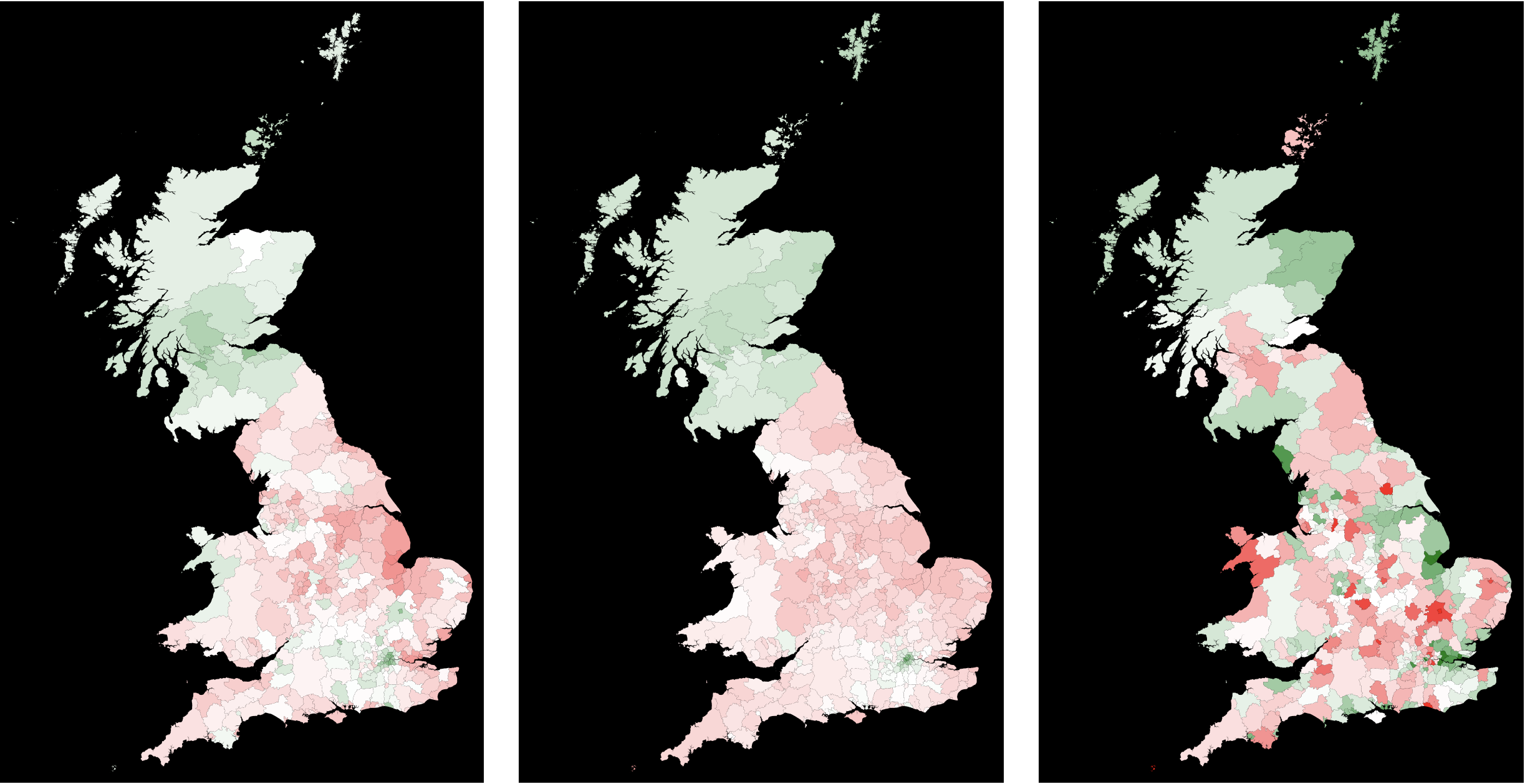
On the left we have the outcome of the elections. In the middle we represent the estimate of the remain/leave ratio based on our linear model. The right figure shows the size of the "correction". The model shows a strong separation between Scotland and most regions in England. The exception in England is the region around London.
Area weighted model
Next we will pool the different regions to better understand regional difference.
codepercent = Transpose[{inputLinearModelcompletewRcode[[All, 1]], MapThread[lmodelfulldata, Transpose[inputLinearModelcompletewRcode[[All, 2 ;; -2]]]]}]
We basically set all the inputs to zero apart from the region data
codepercentregion =
  Transpose[{inputLinearModelcompletewRcode[[All, 1]],
    MapThread[lmodelfulldata,
     Transpose[(Flatten /@
         Transpose[{inputLinearModelcompletewRcode[[All, 1 ;; 2]],
           ConstantArray[0, {382, 6}]}])[[All, 2 ;; -2]]]]}];

GraphicsRow[{Graphics[
   Flatten[Table[{ColorData[
        "RedGreenSplit"][((Select[
             Select[votingData[[2 ;;]], #[[1]] < 381 &], #[[4]] ==
               translateshpvoteclean[[k, 2]] &][[1]])[[-3]]/100.)],
      localauthorities[[1, 2, 1, 2, 1, 2, 1, 1, 1]][[k]]}, {k, 1,
      380}], 1], Background -> Black, AspectRatio -> GoldenRatio],
  Graphics[Table[{ColorData["RedGreenSplit"][
      1 - (((If[# == {}, {Select[
                   votingData, #[[4]] ==
                    translateshpvoteclean[[k, 2]] &][[1, {4, -2}]]/{1,
                   100.}}, #] &@
             Select[codepercentregion, #[[1]] ==
                translateshpvoteclean[[k, 2]] &])[[1]])[[-1]])],
     localauthorities[[1, 2, 1, 2, 1, 2, 1, 1, 1]][[k]]}, {k, 1,
     Length[translateshpvote]}], Background -> Black,
   AspectRatio -> GoldenRatio],
  Graphics[Flatten[
    Table[{ColorData[
        "RedGreenSplit"][(0.5 +
         3.*((1 - (((If[# == {}, {Select[
                    votingData, #[[4]] ==
                    translateshpvoteclean[[k, 2]] &][[1, {4, -2}]]/{1,
                     100.}}, #] &@
                    Select[
                    codepercentregion, #[[1]] ==
                    translateshpvoteclean[[k, 2]] &])[[

                  1]])[[-1]])) - (((If[# == {}, {Select[
                    votingData, #[[4]] ==
                    translateshpvoteclean[[k, 2]] &][[1, {4, -2}]]/{1,
                     100.}}, #] &@
                   Select[
                    Select[
                    votingData[[2 ;;]], #[[1]] < 381 &], #[[4]] ==
                    translateshpvoteclean[[k, 2]] &])[[1]])[[-3]]/
              100.)))],
      localauthorities[[1, 2, 1, 2, 1, 2, 1, 1, 1]][[k]]}, {k, 1,
      380}], 1], Background -> Black, AspectRatio -> GoldenRatio]},
 ImageSize -> Full]
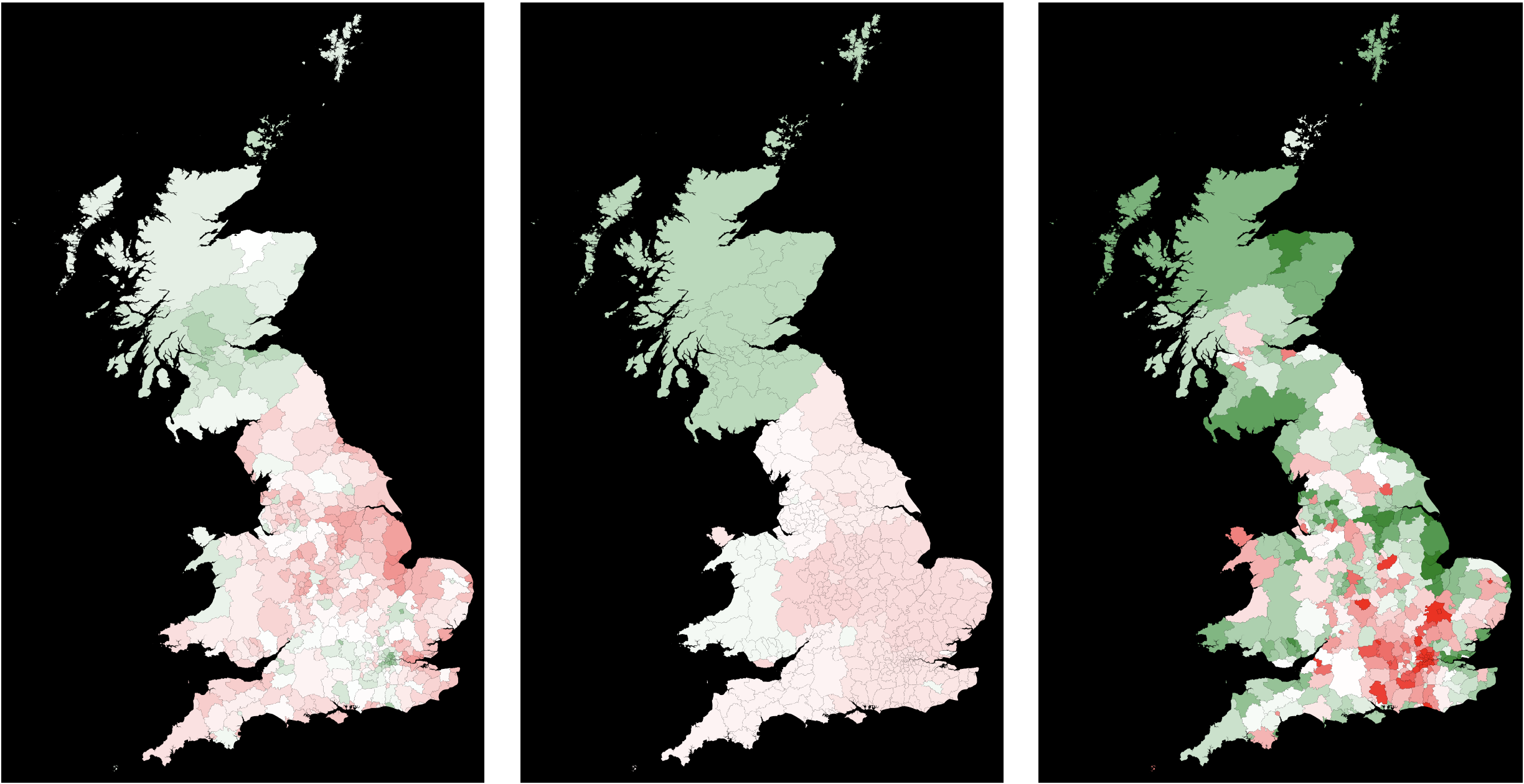
This provides the smoothed picture as regions are pooled and weighted according to their representation in the UK. As before the leftmost image represents the outcome of the election, the middle one is the best region weighted estimate and the right figure shows the differences. The strong divide between the different regions is enhanced in this representation.
Population weighted representation
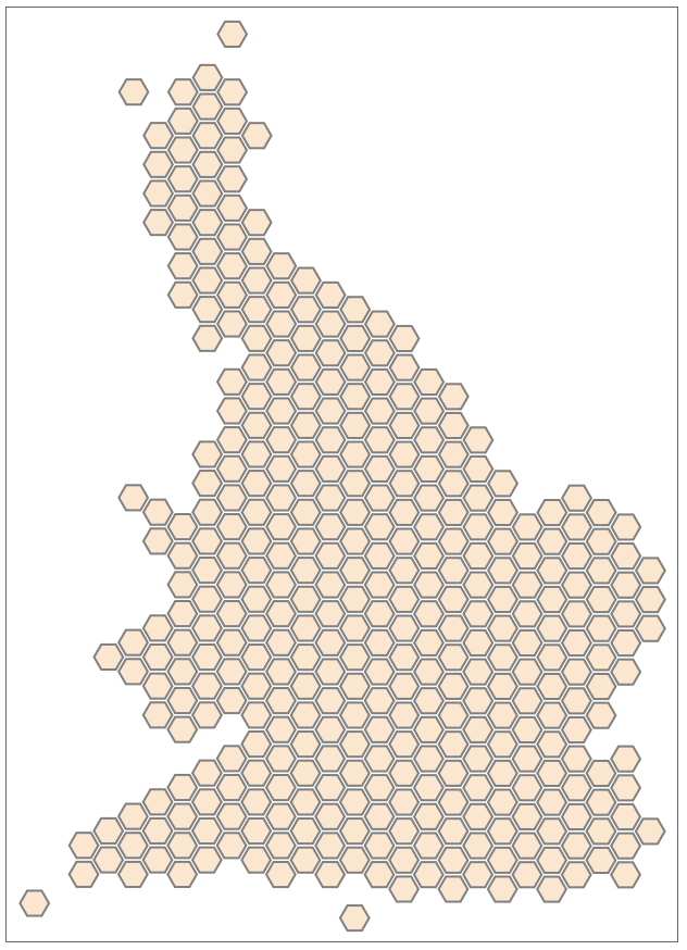
The representations above have the critical drawback that equal area sizes do not necessarily correspond to equally sized electorates. We can represent everything such that area corresponds to population size. This will decrease the size of the regions with low population densities such as Scotland. The following file (attached) contains a hexagonal lattice that describes the areas in the UK.
hexagonshape = Import["GB_Hex_Cartogram_LAs.shp"]
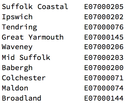
The following file contains a lookup table of regions vs area codes.
hexagonlegend = Import["GB_Hex_Cartogram_LAs.dbf"];
hexagonlegend[[1 ;; 10, {3, 2}]] // TableForm
We now need to translate between the hexagonal structure and the voting areas from our model.
tranlatehexagonvoteclean =
  Table[Select[hexagonlegend, #[[2]] == translateshpvoteclean[[i, 2]] &], {i, 1,Length[translateshpvoteclean]}][[All, 1, 1]];
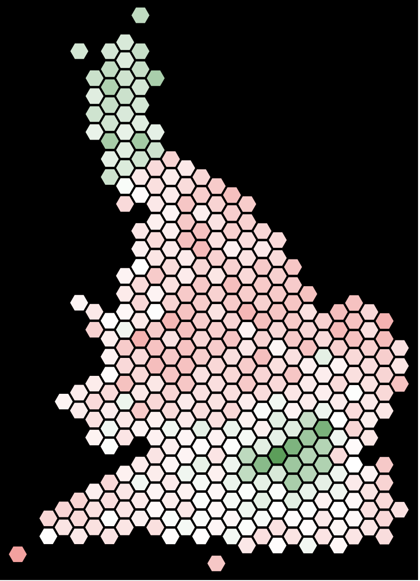
We can then represent the estimate from our model in an population/area adjusted representation.
Graphics[Table[{ColorData["RedGreenSplit"][1 - (( If[# == {}, {Select[votingData, #[[4]] ==
translateshpvoteclean[[k, 2]] &][[1, {4, -2}]]/{1, 100.}}, #] &@
Select[codepercent, #[[1]] == translateshpvoteclean[[k, 2]] &])[[1]][[-1]]) /. Missing[] -> 0.],
 hexagonshape[[1, 2, 1, 2]][[tranlatehexagonvoteclean[[k]]]]}, {k, 1, Length[tranlatehexagonvoteclean]}], Background -> Black]
Preliminary summary
These calculations show that we might have to perform some sort of estimation procedure to better understand the "will of the people". The method we have used is quite standard in for example medical studies. This is, however, not a suitable way of decision making in societies. As said many times before, the decision is based on an agreed upon procedure. It is not based on a statistical analysis of the data, which as in our case is model dependent.
Bootstrapping ----------
Note, that there are different approaches to try to mathematically guesstimate what the people who did not vote think about Brexit. Alternatively to the method described above we could pool all data from all local authorities and scale up to the entire electorate (unnecessary) and bootstrap on that.
The argument of many politicians would be that the non-voters essentially behave like the voters. In that case we basically scale up the results from the voters to the entire electorate. The bootstrapping in this case would look like this:
Monitor[fullpoolresults =
   Table[Count[RandomChoice[Total /@ Transpose[{N@#[[13]]/#[[11]]*#[[6]], #[[6]] - N@#[[13]]/#[[11]]*#[[6]]} & /@ (Reverse@
   SortBy[votingData[[2 ;;]], #[[9]] &])] -> {"Leave", "Remain"}, 46500001], "Remain"]/46500001., {i, 1, 100}];, i]
We can fit a smooth kernel distribution to the outcomes of the bootstrapping procedure:
distfullpool = SmoothKernelDistribution[fullpoolresults]
As expected the probability that more than 50% of the electorate would have wanted to Remain is (numerically) zero.
Probability[x > 0.50, x \[Distributed] distfullpool]
(*0*)
So, under this model assumption it is certain that people really wanted Brexit.
The assumption that the electorate is that homogeneous is quite questionable. We might therefore choose to bootstrap with respect to the local authorities. In other words, we assume that it is on the authority level that voters are similar.
Monitor[localauthresults =
   Table[N@(Total[#[[All, 13]]/#[[All, 11]]*#[[All, 6]]]/
         Total[#[[All, 6]]]) &@
     RandomChoice[(Reverse@SortBy[votingData[[2 ;;]], #[[9]] &])[[All,
         6]] -> (Reverse@SortBy[votingData[[2 ;;]], #[[9]] &]),
      Length[votingData[[2 ;;]]]], {i, 1, 1000}], I];
This bootstraps for the percentage of Remain votes. We can then again fit a distribution:
distlocalauthorities = SmoothKernelDistribution[localauthresults]
and plot the result:
Plot[PDF[distlocalauthorities, x], {x, 0.45, 0.55}, PlotRange -> All,
 FrameLabel -> {"percent leave", "probablity density"},
 LabelStyle -> Directive[Bold, 18], ImageSize -> Large,
 PlotTheme -> "Marketing"]
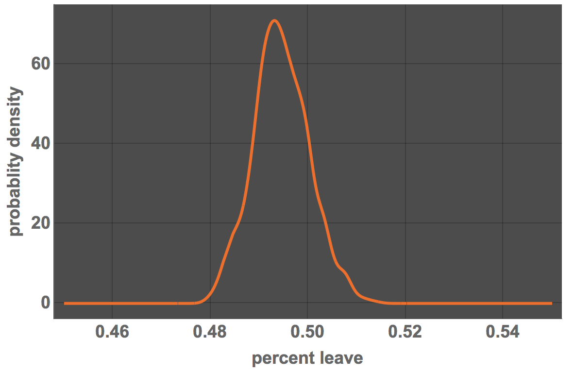
This means that the average of the bootstrap results for Remain votes is below 50%.
Mean[distlocalauthorities]
0.494498. This is, however, quite close to 50%. There is a substantial area above the 50% level:
Probability[x > 0.50, x \[Distributed] distlocalauthorities]
0.17122. This suggests that there is a 17% probability that the voter actually wanted to tell us that they want to remain. This is a substantial fraction/probability. Under these assumptions it is by no means clear that the electorate wanted to leave. Once again, this is not how we take democratic decisions. The decision making process is determined by the outcome of the election and not by an estimate of the voters' will. The point is that it is questionable whether politicans can claim that the voters' will is clear.
The last approach is to bootstrap over the local authorities according to the number of ballots cast:
localvotersresults =
  Table[N@(Total[#[[All, 13]]]/Total[#[[All, 11]]]) &@RandomChoice[(Reverse@SortBy[votingData[[2 ;;]], #[[9]] &])[[All, 11]] -> (Reverse@SortBy[votingData[[2 ;;]], #[[9]] &]), Length[votingData[[2 ;;]]]], {10000}];
Once more we estimate the distribution:
localvotersdist = SmoothKernelDistribution[localvotersresults]
and plot the resulting probability density function:
Plot[PDF[localvotersdist, x], {x, 0.45, 0.55}, PlotRange -> All,
 FrameLabel -> {"percent leave", "probablity density"},
 LabelStyle -> Directive[Bold, 18], ImageSize -> Large,
 PlotTheme -> "Marketing"]
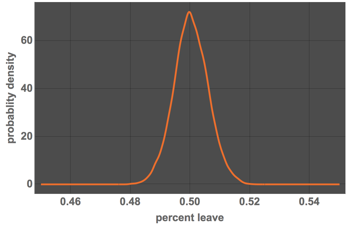
Probability[x < 0.50, x \[Distributed] localvotersdist]
0.487381. So under this assumption we would interpret the voters' will as nearly completely undecided. There is a 50%/50% split, i.e. it is practically equally likely that the voters wanted to remain as that voters wanted to leave.
Conclusion
"The will of the voters" is difficult to understand in close elections. It is by no means as clear that the winning alternative of an election represents the "will of the people" when elections are very close. Politicians often like to stress that they represent the will of the people after winning an election. Mathematically speaking, this is not necessarily true. Note, that this is irrelevant for the decision making process. As a society we have decided to abide by fixed electoral rules. Only people who actually vote will make their voices heard. We can mathematically try to figure out what the entire electorate wanted, or to be precise make probability statements about what they wanted. These statements are clearly model dependent.
 Attachments: