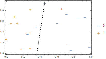
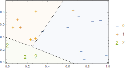
Here' s a diagram we often see in machine learning. I want to construct something like it using the Wolfram Language and Classify, at least when the method is logistic regression. Here's how I go about it.

Let' s generate some simple data.

 SeedRandom[121217];
 trainx = RandomReal[{0, 1}, {20, 2}];
 trainy = Map[
    If[LogisticSigmoid[{-2.7, 1.4}.# + 
         RandomVariate[NormalDistribution[0.3, 0.5]]] > 0.5, 1, 0] &, 
    trainx];

If our classification task does not require much complexity, we can use LogitModelFit and some algebra to find the boundary.

boundaryExpression[fm_FittedModel] := 
  y /. Quiet@First@Solve[fm[x, y] == 1/2, y] // Expand;
boundaryExpression[lomf]

We find it is y=-3.69718 + 10.2671 x

We can now visualize the boundary and get a picture like the one above with the following code.

 With[{be = boundaryExpression[lomf]}, 
  Show[ListPlot[
    KeySort[GroupBy[
      MapThread[List, {trainx, trainy}], (ToString[Last[#]] &) -> 
       First]], PlotMarkers -> {{"-", 18}, {"+", 18}}, Axes -> False, 
    Frame -> True], 
   Plot[be, {x, 0, 1}, PlotStyle -> {Thick, Dashed, Black}]]

But all of that is using LogitModelFit. Sometimes we need regularization or other features of Classify. So, here's how we generate a similar picture using Classify.

 cl = Classify[trainx -> trainy, Method -> {"LogisticRegression", "L1Regularization" -> 0, 
 "L2Regularization" -> 0}, TrainingProgressReporting -> None];

We get the probabilities for each class.

 ci = ClassifierInformation[cl, "ProbabilitiesFunction"]

This generates a function that produces an Association:

 Association[{0 -> (0.0307046 E^(8.58421 #1))/(
     0.0307046 E^(0. + 8.58421 #1) + 0.675585 E^(0.836087 #2)), 
    1 -> 1./(1. + 0.0454489 E^(8.58421 #1 - 0.836087 #2))}] &

We can again use a little algebra to find the boundary.

 boundaryExpression[a_Function] := 
   y /. Quiet@
     First@Simplify[Solve[Equal @@ a[x, y], y, Reals], 
       x \[Element] Reals];
 boundaryExpression[cl_ClassifierFunction] := 
  boundaryExpression[
   ClassifierInformation[cl, "ProbabilitiesFunction"]]

We can now use this function to make a plot quite similar to the one above.

 With[{be = boundaryExpression[cl]}, 
  Show[ListPlot[
    KeySort[GroupBy[
      MapThread[List, {trainx, trainy}], (ToString[Last[#]] &) -> 
       First]], PlotMarkers -> {{"-", 18}, {"+", 18}}, Axes -> False, 
    Frame -> True], 
   Plot[be, {x, 0, 1}, PlotRange -> {{0, 1}, {0, 1}}, 
    PlotStyle -> {Dashed, Black}]
   ]
  ]

Here's another way that does not require use of algebra. Instead we rely on RegionPlot and Ordering.

 Show[ListPlot[
   KeySort[GroupBy[
     MapThread[List, {trainx, trainy}], (ToString[Last[#]] &) -> 
      First]], PlotMarkers -> {{"-", 18}, {"+", 18}}, Axes -> False, 
   Frame -> True], 
  RegionPlot[
   Ordering[ci[x, y], -1][[1]] == 1, {x, 0 - 1, 2}, {y, -1, 2}, 
   PlotRange -> {{0, 1}, {0, 1}}, BoundaryStyle -> {Dashed, Black}, 
   PlotStyle -> {Opacity[0], White}]
  ]

By using RegionPlot we can readily extend the production of boundary diagrams to situations involving more than two classes.

 cl3 = Classify[trainx -> trainy2, 
    Method -> {"LogisticRegression", "L1Regularization" -> 0, 
      "L2Regularization" -> 0}, TrainingProgressReporting -> None];
 ci3 = ClassifierInformation[cl3, "ProbabilitiesFunction"];
 c3plot = Show[
   ListPlot[KeySort[
     GroupBy[MapThread[List, {trainx, trainy2}], (ToString[Last[#]] &) -> 
       First]], PlotMarkers -> {{"-", 18}, {"+", 18}, {"2", 18}}, 
    Axes -> False, Frame -> True], 
   RegionPlot[{Ordering[ci3[x, y], -1][[1]] == 1, 
     Ordering[ci3[x, y], -1][[1]] == 2, Ordering[ci3[x, y], -1][[1]] == 3}, {x,
      0 - 1, 2}, {y, -1, 2}, PlotRange -> {{0, 1}, {0, 1}}, 
    BoundaryStyle -> {{Dotted, Black}}, PlotStyle -> {Opacity[0.05]}]
   ]

I attach a notebook that recapitulates this post and adds an animation.