1) Are you looking to find
$$f(x) \approx \sum_j a_j \phi(x - x_j)$$
where
$\phi(x) = \exp(-(b/h^2)\,x^2)$, where
$b > 0$ is a parameter and
$h$ is the distance between the evenly spaced centers
$x_j$? (A linear problem.)
If RBF interpolation is the sort of thing you want, the approach of Boyd & Wang (2009) seems easy to program (eq. (38)), assuming it's easy to determine when to truncate the series and the parameters
$b$ (
$=\alpha^2$ in Boyd & Wang) and
$h$. It seems to approximate an RBF interpolation with extremely good error properties. The approximation (eq. (12)) is obtained by approximating the Fourier Transform (eq. (9)) of the "cardinal function" for RBF interpolation, taking the inverse transform and approximating it as well.
2) Or will
$b = b_j$ be different at each center and optimized? (A nonlinear problem.)
3) Or will the centers be irregularly spaced?
4) How many centers do you think you might need? (This might determine whether a dumb method can be used on a small number of centers, or an efficient method is needed.)
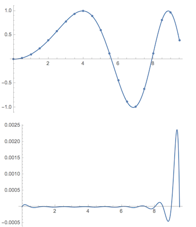
Here's what is surely a "dumb method" for problem 2) above, or at least a naive one. But the result is not too bad on this example.
(* data from Peter's linked example *)
Ndata = 20;
x = Table[10 N[{i/Ndata}], {i, 0, Ndata - 1}];
y = Sin[0.1 x^2];

model = Sum[a[i] Exp[-b[i] (t - x[[i, 1]])^2], {i, 1, Length@x, 2}];  (* one Gaussian per pair *)
nlm = NonlinearModelFit[
  Transpose[Join[Transpose[x], Transpose[y]]],
  model,
  Transpose[{  (* parameters + initial values *)
    Join[Array[a, Length@x][[;; ;; 2]], Array[b, Length@x][[;; ;; 2]]],
    Join[Flatten@y[[;; ;; 2]], ConstantArray[0.5, Length@x][[;; ;; 2]]]
    }],
  t, MaxIterations -> 1000]

nlm["BestFitParameters"]
(*
{a[1] -> 23.1599, a[3] -> -13.0745, a[5] -> 0.73477,
 a[7] -> 0.0989986, a[9] -> 0.155762, a[11] -> 0.0914005,
 a[13] -> -9.50923, a[15] -> -2.4148, a[17] -> 0.392815,
 a[19] -> 1.76915, b[1] -> 0.008367, b[3] -> 0.028266,
 b[5] -> 0.123698, b[7] -> 0.544691, b[9] -> 0.595277,
 b[11] -> 0.599547, b[13] -> -0.00378785, b[15] -> 0.289993,
 b[17] -> 0.797485, b[19] -> 0.685441}
*)
For inspecting accuracy:
Show[
 Plot[nlm[t], {t, 0, 9.5}],
 ListPlot[Transpose[Join[Transpose[x], Transpose[y]]]],
 PlotRange -> All
 ]

Plot[nlm[t] - Sin[0.1 t^2], {t, 0, 9.5}, PlotRange -> All]