If I understand correctly, you can get a Riemann approximation to what you want just by taking partial sums with Accumulate.
ListPlot[Transpose[{evals[[1, All, 1]], Accumulate[evals[[1, All, 2]]]}]]
This is not so accurate though. Perhaps better, if somewhat cumbersome, is to gather the sampling points as you already do, order them, then redo the integrations between consecutuve pairs thereof. Accumulating these subinterval integrals will give the picture I think you are after. Here is the idea.
(* repeat code from original post *)
rulePoints = 5;
sampledPoints =
  Reap[NIntegrate[(0.00159155/(x^2 + 0.000025^2)), {x, -10, 10},
     Method -> {"LocalAdaptive", "SymbolicProcessing" -> 0,
       Method -> {"TrapezoidalRule", "Points" -> rulePoints},
       "SingularityHandler" -> None}, EvaluationMonitor :> Sow[x]]][[2, 1]];

(* Now integrate between sampled points *)
newpoints = Sort[sampledPoints];
ivals = Table[NIntegrate[(0.00159155/(x^2 + 0.000025^2)), {x, newpoints[[i]],
     newpoints[[i + 1]]}], {i, Length[newpoints] - 1}];
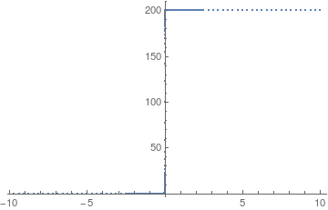
Plot:
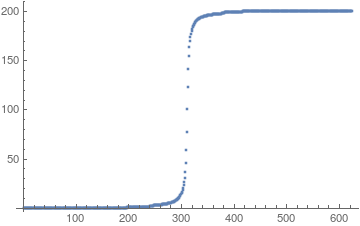
ListPlot[Transpose[{Rest[newpoints], Accumulate[ivals]}], PlotRange -> All]
Maybe slightly better on the eyes:
ListPlot[Accumulate[ivals], PlotRange -> All]