Click on the image to zoom. Then click your browser back button to return to reading the post.

Motivation
It was (correctly) pointed out to me that the ColorFunction I used in my visualization for the DataViz Challenge was not color-blind friendly. The user further linked to an online simulator one could use to check their visualizations. This got me thinking more about the subject and I decided to implement one in the WL. Perhaps I should've checked if such a thing already existed first (does it?), but I learned some exciting stuff along the way nonetheless, I wish to share especially in light of the second Data Viz challenge on Monday.
Spelunking ColorOperationsDump
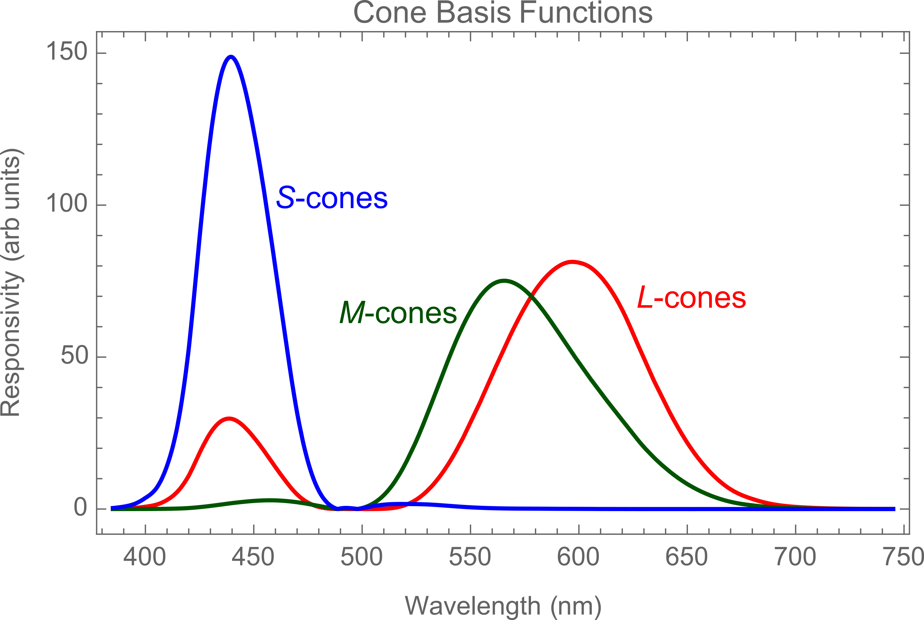
There's a wealth of undocumented functions broadly related to 'color', which can be very useful. For example in understanding the CIE standard observer which is closely related to the concept of spectral cone sensitivity we'll use below.
ChromaticityPlot["RGB"];
{xInt, yInt, zInt} =
  Interpolation[
     Thread[{Image`ColorOperationsDump`$wavelengths, #}]] & /@
   Transpose[Image`ColorOperationsDump`tris];

Plot[{xInt[\[Lambda]], yInt[\[Lambda]], zInt[\[Lambda]]}, {\[Lambda],
  385, 745}, PlotStyle -> {Red, RGBColor[0, 0.33, 0], Blue},
 PlotLabel -> "Cone Basis Functions", Frame -> True,
 FrameLabel -> {"Wavelength (nm)", "Responsivity (arb units)"},
 ImageSize -> Large, BaseStyle -> {FontSize -> 18}]

I used a semi-manual procedure using Information to locate the functions of interest to this project. For example ?-correction and the RGBtoXYZ transformation matrix we'll use below like so:
?Image`ColorOperationsDump`*gamma*
DownValues[Image`ColorOperationsDump`gammaCorrect][[1]]
Image`ColorOperationsDump`RGBtoXYZmatrix["sRGB"]
Color Space Tranformations
Note: I'm actually not sure whether RGBColor[] uses linear RGB values or just scaled sRGBs (clarification would be great). I assumed the latter just to show the test case of applying ?-corrections for completeness. The results don't vary appreciably either way.
In the standard RGB (sRGB) color space, doubling the values of sRGB indicates double the intensity. This makes sense for the case of digital cameras, however our eyes don't work that way. In fact we perceive this doubling as being only fractionally brighter - increasingly so for higher light intensities. I.e. we need to apply a nonlinear correction to 'perceive' the correct color from a digital image. The simplest such case is the power law ?-correction and is given by (compiled for later efficiency):
gammaCorrect = Compile[{{val, _Real, 1}},
   Table[If[i <= 0.0031308, 12.92 i, 1.055 i^0.41666 - 0.055], {i,
     val}], CompilationTarget -> "C", RuntimeOptions -> "Speed"];
Similarly, the inverse function can be used to 'uncorrect' the digital images, like so:
    gammaUncorrect = Compile[{{val, _Real, 1}},
       Table[If[i <= 0.04045, i/12.92 , ((i + 0.055)/1.055)^(
         1/0.41666)], {i, val}], CompilationTarget -> "C",
       RuntimeOptions -> "Speed"];
Once we have our linear RGB values (scaled between 0-1), we can use the undocumented functionality to transfer them into the tristimulus XYZ color space:
MatrixForm[
 M["sRGB" -> "XYZ"] =
  Image`ColorOperationsDump`RGBtoXYZmatrix["sRGB"]]
What we're really interested in however is to move to the LMS color space, since colorblindness is related to cones abnormalities; This is achieved using the Hunt-Pointer-Estevez transformation:
MatrixForm[
 M["XYZ" -> "LMS"] = {{0.4002, 0.7076, -0.0808}, {-0.2263, 1.1653,
    0.0457}, {0, 0, 0.9182}}]
We can of-course combine these into a single transformation, and compute its inverse:
MatrixForm[M["sRGB" -> "LMS"] = M["XYZ" -> "LMS"].M["sRGB" -> "XYZ"]]
MatrixForm[M["LMS" -> "sRGB"] = Inverse[M["sRGB" -> "LMS"]]]
Example usage is therefore as follows for the RGB primitives:
TableForm@
 Table[{RGBColor[i],
   Thread[{{"L :", "M :", "S :"},
     M["sRGB" -> "LMS"].gammaUncorrect[i]}]}, {i, {{1, 0, 0}, {0, 1,
     0}, {0, 0, 1}}}]
Simulating Color Blindness
There are three main types of dichromatic view colorblindness:
- Protanopoia (Red-Green colorblindness with less sensitivity to Red)
- Deuteranopia (Red-Green colorblindness with less sensitivity to Green)
- Tritanopia (Blue-Yellow colorblindness)
Essentially Protanopes are missing L-cones, Deuteranopes are missing M-cones and Tritanopes are missing S-cones. As such, we can simulate their vision by applying a transformation matrix,S to their LMS color values and then translating back to RGB. This can be done as follows: $$M_{LMS->RGB} . S . M_{RGB->LMS}. \left\{R,G,B\right\} = \left\{R',G',B'\right\}$$
It's tempting to merely drop the respective cones for each type of colorblindness (i.e. diagonalize S with a trace of 2), but it turns out we get better results by expressing the missing cones as a linear combination of the other cones like so:
S["protanopes"] = {{0, a, b}, {0, 1, 0}, {0, 0, 1}};
S["deuteronopes"] = {{1, 0, 0}, {a, 0, b}, {0, 0, 1}};
S["tritanopes"] = {{1, 0, 0}, {0, 1, 0}, {a, b, 0}};
We now need to solve for these unknown coefficients for each type. To do so we need two equations, and thus we make two assumpions:
- The 'color' White is not affected for any colorblindness type
- The RGB color furthest from the missing cones' peak is also minimally affected (Blue for protanopes and deuteronopes, Red for tritanopes)
With these two assumptions, we write a function to solve for these coefficients and wrap everything together:
sMatrix[s_, constants_] :=
 s /. First[
   Solve[Join @@
     Table[Thread[s.M["sRGB" -> "LMS"].i == M["sRGB" -> "LMS"].i], {i,
        constants}], {a, b}]]
colorBlindness = Compile[{{transformation, _Real, 2}, {rgb, _Real, 1}},
      Chop[gammaCorrect[transformation.gammaUncorrect[rgb]]],
      CompilationTarget -> "C", RuntimeAttributes -> {Listable},
      RuntimeOptions -> "Speed",
      CompilationOptions -> {"InlineCompiledFunctions" -> True}]
Examples
We can know use our simulator to simulate Lena or the grocery store fruit in the beginning of this post:
GraphicsRow[
 MapThread[(Show[
     Image[Table[
       colorBlindness[sMatrix[#1, #2], i], {i,
        ImageData[ExampleData[{"TestImage", "Lena"}]]}]],
     PlotLabel -> #3]) &, {{{{1, a, b}, {0, 1, 0}, {0, 0, 1}},
    S["protanopes"], S["deuteronopes"],
    S["tritanopes"]}, {{{1, 1, 1}, {0, 0, 1}}, {{1, 1, 1}, {0, 0,
      1}}, {{1, 1, 1}, {0, 0, 1}}, {{1, 1, 1}, {1, 0,
      0}}}, {"Original", "Protanopia", "Deuteranopia",
    "Tritanopia"}}], ImageSize -> 1000]

Color Data
Now, turning to the Built-in color schemes: we'll investigate both the indexed and gradient color schemes. First some wrapper functions to extract the colors in RGB manner:
gradients = ColorData["Gradients"];
indexed = ColorData["Indexed"];
cols[name_] := ColorConvert[Switch[Head[name], Integer,
   ColorData[name, "ColorList"], _, ColorData[name] /@ Subdivide[9]],
  "RGB"]
decapitate[expr_] := Replace[expr, h_[a__] :> {a}, {0, \[Infinity]}]
Contrast Ratio
We need some sort of metric to evaluate these before and after they are color-blind simulated. I chose a contrast ratio of relative luminance (but I welcome other suggestions).
relativeLuminance = Compile[{{rgb, _Real, 1}},
  gammaUncorrect[rgb].{0.2126, 0.7152, 0.0722},
  CompilationTarget -> "C", RuntimeAttributes -> {Listable},
  RuntimeOptions -> "Speed",
  CompilationOptions -> {"InlineCompiledFunctions" -> True}]
contrast = Compile[{{rgb1, _Real, 1}, {rgb2, _Real, 1}},
  Module[{lum1 = relativeLuminance[rgb1],
    lum2 = relativeLuminance[rgb2], sorted},
   sorted = Sort[{lum1, lum2}];
   (sorted[[2]] + 0.05)/(sorted[[1]] + 0.05)],
  CompilationTarget -> "C", RuntimeAttributes -> {Listable},
  RuntimeOptions -> "Speed",
  CompilationOptions -> {"InlineCompiledFunctions" -> True}]
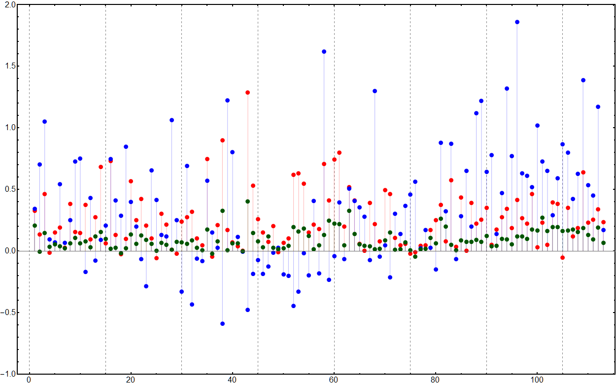
We calculate the mean contrast value for all the colors in a particular color function for each of the colorblindness types and then use the original contrast as a baseline. Negative values therefore show a decrease in contrast after the transformations.
indexedMeans = Block[{pro, deu, tri},
   Table[
    pro =
     colorBlindness[sMatrix[S["protanopes"], {{1, 1, 1}, {0, 0, 1}}],
      decapitate[i]];
    deu =
     colorBlindness[
      sMatrix[S["deuteronopes"], {{1, 1, 1}, {0, 0, 1}}],
      decapitate[i]];
    tri =
     colorBlindness[sMatrix[S["tritanopes"], {{1, 1, 1}, {1, 0, 0}}],
      decapitate[i]];
    TrimmedMean[contrast @@ Transpose[Tuples[#, 2], {2, 1, 3}],
       0.25] & /@ {decapitate[i], pro, deu, tri}, {i,
     cols /@ indexed}]];
visualizationIndexed =
  ListPlot[Transpose[
    MapThread[{#2, #3, #4} - #1 &, Transpose[indexedMeans]]],
   PlotStyle -> {{Red, Thick}, {Blue, Thick}, {RGBColor[0, 0.33, 0],
      Thick}}, Frame -> True, FrameStyle -> Directive[Black, Thick],
   Filling -> Axis, PlotRange -> {-1, 2}, ImageSize -> 1250,
   GridLines -> {Range[0, 113, 15], None},
   GridLinesStyle -> Directive[Gray, Dashed], BaseStyle -> 16]

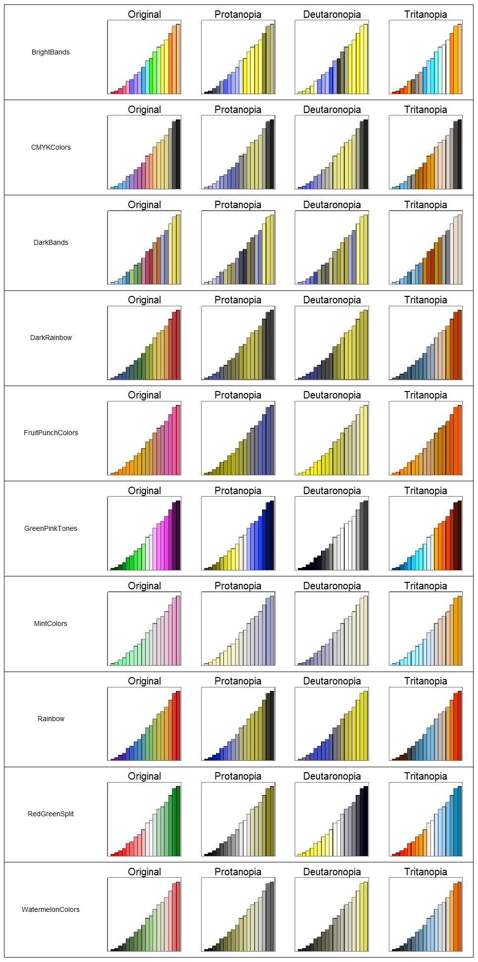
Similarly for the gradients. Unsurprisingly the gradients perform poorer with only ten being color-blind friendly:
unfriendlyGradients =
  With[{asc =
     Last /@ GroupBy[
       Position[
        MapThread[{#2, #3, #4} - #1 &, Transpose[gradientMeans]],
        a_ /; a < 0], First]},
   AssociationThread[gradients[[Keys[asc]]] -> Values[asc]]];
friendlyGradients = Complement[gradients, unfriendlyGradients // Keys]
{"BrightBands", "CMYKColors", "DarkBands", "DarkRainbow", \ "FruitPunchColors", "GreenPinkTones", "MintColors", "Rainbow", \ "RedGreenSplit", "WatermelonColors"}
Visual Testing
Finally, we put the 10 gradients to the test:
barChart[cFun_] := Block[{og, pro, deu, tri},
  og = Rasterize[
    BarChart[
     Partition[Prime[Range[18]], 2], {PerformanceGoal -> "Speed",
      Ticks -> None, Frame -> True, FrameTicks -> None,
      AspectRatio -> 1, ImageSize -> 125, ColorFunction -> cFun}]];
  pro = Image[
    colorBlindness[
       sMatrix[S["protanopes"], {{1, 1, 1}, {0, 0, 1}}], #] & /@
     ImageData[og]];
  deu = Image[
    colorBlindness[
       sMatrix[S["deuteronopes"], {{1, 1, 1}, {0, 0, 1}}], #] & /@
     ImageData[og]];
  tri = Image[
    colorBlindness[
       sMatrix[S["tritanopes"], {{1, 1, 1}, {1, 0, 0}}], #] & /@
     ImageData[og]];
  Prepend[
   MapThread[
    Show[#1, PlotLabel -> Style[#2, Black, 14]] &, {{og, pro, deu,
      tri}, {"Original", "Protanopia", "Deuteranopia",
      "Tritanopia"}}], cFun]]
GraphicsGrid[barChart /@ friendlyGradients, Frame -> {False, True}]

This was a fun exercise into the dark magic realm of color, hopefully it's helpful for future DataViz entries. FYI: This website was a great starting point. Looking forward to hear your thoughts on this!
Cheers,
George