Motivation
Some time ago, my coworker Eila Stiegler was working on her blog about the cool Marathon visualization website. While doing so, she asked me if it is possible to make artistic word clouds, such as the one from the 2017 Champaign-Urbana marathon poster (that hangs on her office door) using the Wolfram Language . With only a few weeks until this year's marathon left, I will give this a try.
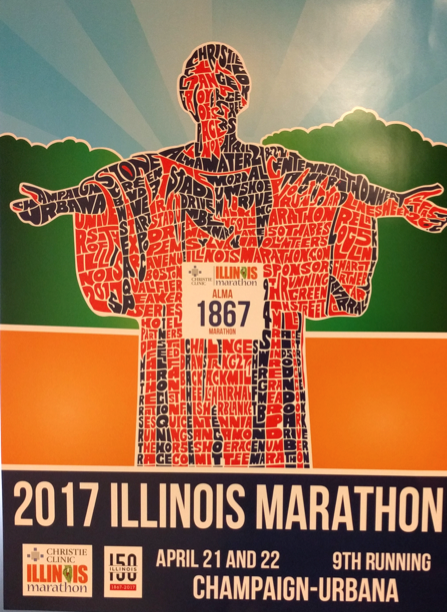
That is an interesting problemhow to make such-type deformed dense letter arrangements in the Wolfram Language.
This hand-made poster has many nice elements, e.g.:
- the words are all contained in the outline of the Alma Mater
- the characters fill out most of the space with smooth outlines, but the character is still recognizable (like in a CAPTCHA)
- the characters of a given word are not all the same size, but the size varies smoothly along a word
- the Illini coloring is correlated to the flow of the robe
To keep this post at reasonable length, let's try to reproduce the first two features: a dense packing of characters that fills a given outer shape.
Our overall approach will be the following:
- make an initial word cloud (using WordCloud) within a given shape (the Alma Mater)
- solve the diffusion equation (using NDSolve) to let the characters of the words diffuse/flow into the space between the words/characters and between the characters and the boundary of the outer shape
- follow the boundaries of the letters under this diffusion process (again using NDSolve)
The use of the diffusion equation to spread out areas was pioneered by Gastner and Newman in building cartograms in their cartogram algorithm. (Because we don't want to preserve the character weights/areas, we will use different boundary conditions.)
If one imagines a liquid with time-and position-dependent concentrations n(t,x,y) of say ink, the ink will spread to a uniform distribution in the long time limit. In our case, the initial letters have a lot of ink and the space between the letters is ink-free.
To follow a single ink molecule, one first solves the classical diffusion equation (with Subscript[c, D] being the diffusion coefficient)

then defines the flow

and then follows that path {x(x),y(t)} of a given inc molecule (in our case character boundary point) with initial position { $x_0,y_0$} through the nonlinear system of ordinary coupled differential equations.
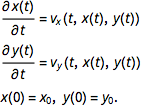
As hinted above, in our example, we will start with a high concentration of ink at the characters and follow the ink molecules that are at the edges of the characters over time.
The individual characters will over time diffuse into the voids between them but they will not start overlapping. And the movement into the voids depends on the available space. So, we expect smooth curves as the boundaries of the spread-out letters. If we would say, use the wave equation instead, we would get interference effects from overlapping waves from the individual characters and the propagation would be uniform in each direction.
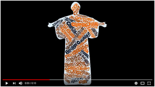
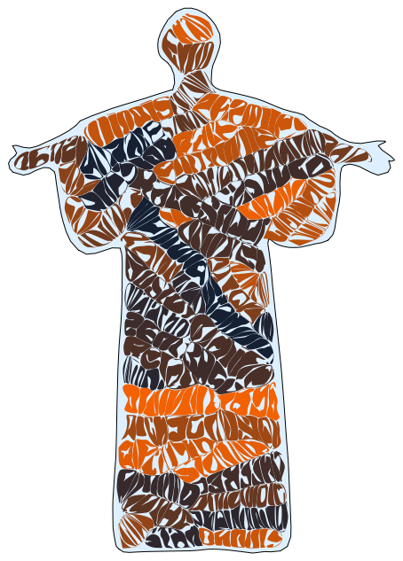
The result will be the following: (click to play)
The Alma Mater Outline
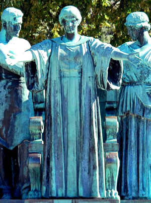
First we need an outline of the outer, word-confining shape. Using a photograph of the Alma Mater, we can quickly trace out the boundary.
Show[ ImageTake[ Import["https://tinyurl.com/yd6dn242"], {220, -500}, {320, -320}], ImageSize -> 300]
almaMater = {{761.7, 1432.}, {790.8, 1425.}, {832.7, 1417.}, {862.3,
    1405.}, {900.7, 1388.}, {928.2, 1386.},
       {946.5, 1364.}, {978.9, 1355.}, {989.5, 1340.}, {1031.,
    1324.}, {1068., 1333.}, {1094., 1333.}, {1075., 1325.},
       {1068., 1321.}, {1108., 1296.}, {1102., 1290.}, {1088.,
    1297.}, {1099., 1285.}, {1093., 1269.}, {1076., 1268.},
       {1071., 1262.}, {1034., 1286.}, {995.5, 1289.}, {1001.,
    1231.}, {990.4, 1183.}, {987.3, 1149.}, {970.6, 1133.},
       {950.2, 1133.}, {929.3, 1126.}, {909., 1123.}, {882.1,
    1127.}, {867.6, 1135.}, {854.8, 1148.}, {865.5, 1072.},
       {874.2, 980.6}, {887.6, 848.7}, {897.3, 709.4}, {900.9,
    629.1}, {906.5, 537.5}, {866.6, 528.8}, {857.9, 533.3},
       {833.4, 528.7}, {814.1, 530.2}, {776.2, 535.9}, {747.6,
    537.4}, {710.3, 532.3}, {675.2, 533.8}, {632.2, 530.7},
       {607.7, 532.3}, {590.4, 528.7}, {558.3, 533.3}, {554.7,
    619.4}, {563.4, 710.6}, {564.1, 825.9}, {568.2, 931.9},
       {575.9, 1021.}, {574.4, 1114.}, {571.3, 1129.}, {542.1,
    1120.}, {513., 1109.}, {495.2, 1113.}, {473.8, 1132.},
       {457.9, 1176.}, {445.6, 1250.}, {444.1, 1280.}, {415.6,
    1281.}, {385., 1262.}, {376.4, 1269.}, {361.7, 1269.},
       {353.5, 1282.}, {350.4, 1292.}, {375.5, 1309.}, {358.6,
    1320.}, {361.9, 1328.}, {390.9, 1314.}, {432.9, 1332.},
       {458., 1345.}, {488.7, 1362.}, {486.7, 1371.}, {528.1,
    1386.}, {555.8, 1396.}, {593.7, 1407.}, {639.6, 1421.},
       {660., 1430.}, {678.8, 1431.}, {676.4, 1454.}, {676.3,
    1463.}, {665.7, 1485.}, {657.6, 1487.}, {643.4, 1502.},
       {643.5, 1532.}, {654.2, 1554.}, {670.4, 1580.}, {693.5,
    1594.}, {726.7, 1588.}, {749.9, 1568.}, {766.9, 1542.},
       {765.8, 1521.}, {761.2, 1504.}, {752.6, 1484.}, {748.2,
    1473.}, {748.2, 1450.}, {747.5, 1440.}, {761.7, 1432.}};

Graphics[FilledCurve[BSplineCurve[almaMater]]]

For the use in WordCloud, we make mask that is exactly this shape.
Show[almaMaterPolygon = Rasterize[Graphics[Polygon[
     Table[
      Evaluate[BSplineFunction[almaMater, SplineDegree -> 2][t]] - {750,
        1000}, {t, 0, 1, 1/200}]]], "Image", ImageSize -> 800],
 ImageSize -> 300]

Making the Word Cloud of Marathon Words
Next, we collect a set of words that describe the Illinois Marathon. Making a web search for pages that mention the marathon event or the twin city might give us some suggestions for words to include.
sites = Function[searchTerm,
    WebSearch[searchTerm,
     MaxItems ->
      25]] /@  {"Illinois marathon",  "Champaign marathon", "Urbana marathon", "Champaign-Urbana"};

urls = Union[Flatten[Normal[#[All, "Hyperlink"]] & /@ sites]];
Monitor[pageData = Table[Import[urls[[j, 1]]], {j, 1 Length[urls]}]; // Quiet, j]

words = KeySelect[
   Select[WordCounts[
     DeleteStopwords[
      StringJoin[Riffle[ToLowerCase[Cases[pageData, _String]], " "]]]], # >=
      50 &], StringLength[#] > 2 &];

WordCloud[words, PlotTheme -> "Monochrome"]

We include the word 'cold', as it was a fresh morning at last year's race.

So, in the following we will use this list of words.
words = {"Marathon", "26.2\[ThinSpace]miles", "42.195\[ThinSpace]km",
   "Champaign", "Urbana", "4\[ThinSpace]hours", "5\[ThinSpace]k",
   "10\[ThinSpace]k",
   "46112\[ThinSpace]y", "138336\[ThinSpace]ft", "Walk", "2017",
   "26\[ThinSpace]mi 385\[ThinSpace]y", "Battle of Marathon", "Half",
   "7\[ThinSpace]am",
   "\[TildeTilde]2,600\[ThinSpace]Cal", "9th Race", "Memorial Stadium",
   "Dick Beardsley", "Sunny", "Rainy", "Windy",
   "Cold", "Warm", "Fun", "9\[ThinSpace]min/mile", "490\[ThinSpace]BC",
   "Race", "Running", "Pheidippides", "April\[ThinSpace]21,22", "Pacers",
   "Christie",
   "Illinois", "Start", "Expo", "Alma Mater", "02:22:18", "Stadium", "Relay",
   "Olympic 1896", "Abe's Log", "BIB", "Race Street", "Green Street",
   "Boston Qualifier", "Winner"};
We use selected seed values to obtain a word cloud that has some words in the head and so that all characters are strictly contained in the Alma Mater. Different seeds will result in different-looking word clouds.
SeedRandom[111]
WordCloud[(RandomReal[{1, 2}] -> #) & /@
  words,
 ColorNegate@almaMaterPolygon, WordOrientation -> {-Pi/3, Pi/3},
 MaxItems -> \[Infinity], ColorFunction -> (Black &), FontSize -> {5, 15},
 RandomSeeding -> 111]
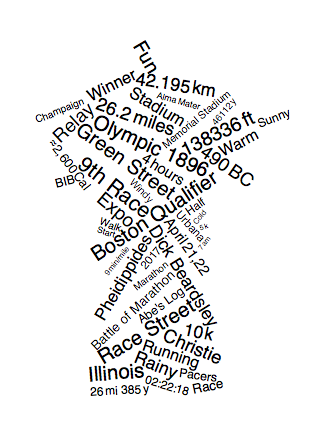
To avoid any dependence of the following calculations and visualisations, here is the word cloud that we want to use in the following (obtained with the seeds 35, 35).

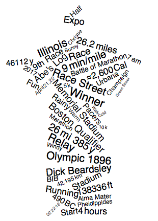
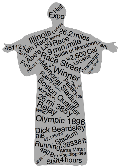
Here are the words from the word cloud within the Alma Mater.
With[{d = ImageSize -> ImageDimensions[almaMaterPolygon]},
 Overlay[{Show[almaMaterPolygon, d],
    Show[SetAlphaChannel[Show[wc1, d],
              Darker@ColorNegate[almaMaterPolygon]], d]}] //

  Rasterize[#, "Image", ImageSize -> 400] &]
Build a Region-object for the Words in the Alma Mater
As we want to solve the diffusion equation, we build a region-object to use in the numerical differential equation solver. We want the characters to have a high initial value and have the characters flow out. To get a good numerical solution, we want a fine grid near the boundaries of the characters that form the words.
We load the FEM package to have such useful functions such as ToElementMesh at our disposal.
Needs["NDSolve`FEM`"]
The characters from the word cloud taken out. Using a larger image size will give later smoother-looking characters. But it will also increase the computation time.
Show[im = ImageMesh[ras = Rasterize[wc1, "Image", ImageSize -> 800]],
 Frame -> True]
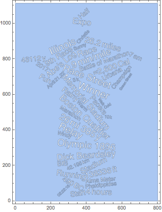
The Alma Mater region mask:
Show[im2 = ImageMesh[ImageResize[almaMaterPolygon,
    ImageDimensions[ras]]], Frame -> True]
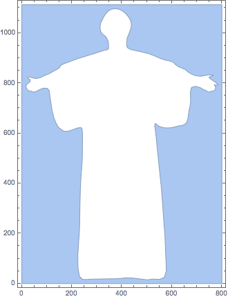
And here are the characters taken out of the Alma Mater region.
im3 = RegionDifference[im, im2]
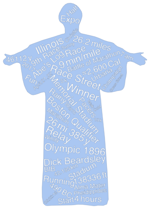
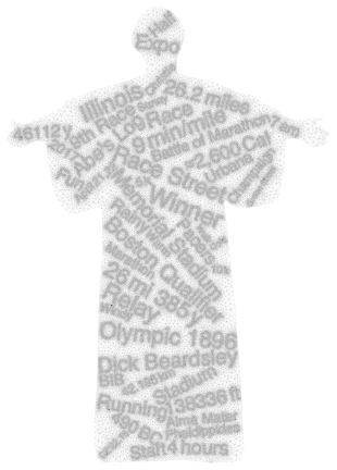
Next, we build the triangulated version for use in the PDE solving. We see the fine triangulation near the character boundaries that we want for an accurate solution of the PDE.
holes = im3["RegionHoles"];
(em = ToElementMesh[RegionBoundary[im3],
     "RegionMarker" -> ({#, 0, 1} & /@ holes), "MaxCellMeasure" -> 100])[
  "Wireframe"] /.                              {e_EdgeForm :>
   EdgeForm[{Black, Thickness[0.0001]}]}
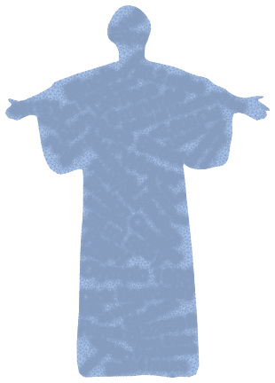
The corresponding mesh region.
mr = MeshRegion[em]
And these are the meshed versions of the individual characters.
outer = Rectangle @@ Transpose[RegionBounds[im]];
Show[allChars =
  RegionDifference[outer, im] // DiscretizeRegion[#, MaxCellMeasure -> 5] &,
 Frame -> True]
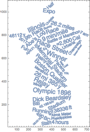
Length[chars = ConnectedMeshComponents[allChars]]
371
Right now, about 21 % of the area of the Alma Mater are occupied by the characters.
Quantity[100 Total[Area /@ chars]/Area[mr], "Percent"] // NumberForm[#, 4] &
21.22%
Colors the Words of the Word Cloud
We want to color each word individually. By overlaying the region characters with the original word cloud, we identify which characters belong to the same word.
We use standard Illini colors.
uOfIColors = {RGBColor[19/255, 31/255, 51/255],
   RGBColor[250/255, 99/255, 0/255]};

SeedRandom[25];
Show[rasC =
  Rasterize[wc1 /. GrayLevel[0] :> Blend[uOfIColors, RandomReal[]], "Image",
   ImageSize -> 800], ImageSize -> 300]
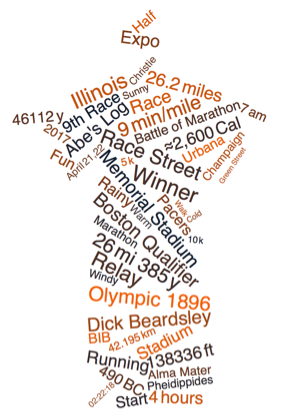
imC = Reverse@ImageData[rasC];

getColor[cm_] :=
 Module[{xMin, xMax, yMin, yMax, reg, points, ccs},
  {{xMin, xMax}, {yMin, yMax}} = RegionBounds[cm] ;
  reg = RegionMember[cm];
  points =
   Cases[Table[
     If[reg[{x, y}], {x, y}, Null], {x, Floor[xMin], Ceiling[xMax]}, {y,
      Floor[yMin], Ceiling[yMax]}], {_, _}, {-2}];
  (* majority color *)
  ccs = DeleteCases[Reverse[SortBy[Tally[
       imC[[Sequence @@ Reverse[#]]] & /@ points], Last]], {{1.`, 1.`,
      1.`}, _}];
  ccs[[1]]]

Monitor[charColors = Table[getColor[chars[[j]]],
                                                      {j, Length[chars]}];, j]
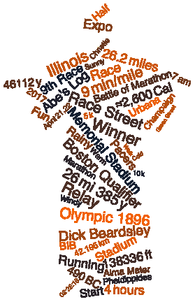
Here are the characters, as regions, colored.
Show[Table[
  Region[chars[[j]], BaseStyle -> {RGBColor @@ charColors[[j, 1]]}], {j,
   Length[chars]}]]
Make Triangles and Region Functions
We extract the triangles from the mesh for the construction of the initial conditions that will be needed in the next section.
triangles = (MeshPrimitives[mr, 2] /.

    Region`Mesh`Quadratic[Polygon[{p1_, p2_, p3_, ___}]] :>
     Polygon[{p1, p2, p3}]);
We have about 240k triangles in our FEM mesh.
Length[triangles]
243642
We calculate the areas and centroids of these triangles.
{centroids, areas} =
  Transpose[{RegionCentroid[#], Area[#]} & /@ Take[triangles, All]];
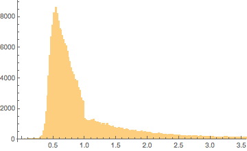
Here is a distribution of the sizes of the triangles from the mesh.
Histogram[areas, 5000]
rb = RegionBoundary[mr];

rd = RegionDistance[allChars];
srd = SignedRegionDistance[mr];
Reconstructing Deformed Characters from Their Boundary Points
As a small intermezzo, and because we will need it later anyway, we implement a function that given a 2D mesh region and a function that maps these points to new (evolved) points, builds filled curves. We do need this function because we want smoothed boundaries and filling of our character outlines. Most of the code deals with detecting interior holes and the order of the points. If we have characters with 'holes' (e.g. A, B), we will actually draw multiple filled curves. First we will draw the outermost one, and then the inner holes with the color of the outer environment on top.
makeClosedCurve[mr_MeshRegion, f_] :=
 Module[{coords, newCoords, lines, gr, orderPoints, fun},
  coords = MeshCoordinates[mr];
  newCoords = f /@ coords;
  lines = MeshCells[mr, 1] /.
    Region`Mesh`Quadratic[Line[{p1_, p2_, _}]] :> Line[{p1, p2}];
  (* order points *)
  gr = Graph[UndirectedEdge @@@ lines[[All, 1]]];
  orderPoints = FindHamiltonianPath[gr];
  fun = BSplineFunction[Append[#, First[#]] &@newCoords[[orderPoints]],
    SplineDegree -> 3 (* could use  SplineClosed \[Rule] True *)];
  Line[Table[fun[s], {s, 0, 1, 1/360}]] ]

makeFilledCurve[mr_MeshRegion, f_, {col1_, col2_}] :=
 Module[{cmcs, cmcs3},
  cmcs = ConnectedMeshComponents[RegionBoundary[mr]];
  Which[Length[cmcs] === 1, {col1,
    FilledCurve[{makeClosedCurve[cmcs[[1]], f]}]},
               Length[cmcs] > 1,
                cmcs3 =  Reverse[SortBy[cmcs, ArcLength]];
               {col1, FilledCurve[ makeClosedCurve[cmcs3[[1]], f]],
                col2, FilledCurve[makeClosedCurve[#, f]] & /@ Rest[cmcs3]}
            ]]
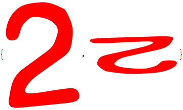
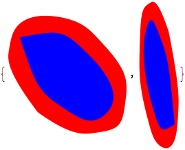
Two examples. With and without holes.
{Graphics[makeFilledCurve[chars[[5]], Identity, {Red, Blue}]],
 Graphics[makeFilledCurve[chars[[5]], -CubeRoot[#] &, {Red, Blue}]]}
{Graphics[makeFilledCurve[chars[[1]], Identity, {Red, Blue}]], Graphics[makeFilledCurve[chars[[1]], -CubeRoot[#] &, {Red, Blue}]]}
Construct the Initial Conditions for the Diffusion Equation
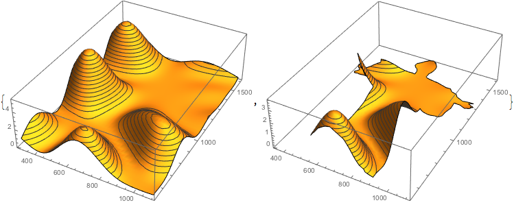
To get some kind of randomness, we construct a random wavy function that determines the initial height of the characters. The height represents the initial 'ink concentration'. This means by using different concrete realizations of the function wavy will result in different final diffused word clouds.
Here is a plot of the initial concentration within the bounding rectangle as well as in the Alma Mater.
SeedRandom[40];
wavy[{x_, y_}] =
  With[{S = 1000, M = 12},
   Sum[RandomReal[{-1, 1}] Cos[x/S RandomReal[{-M, M}] +
         2 Pi RandomReal[]] Cos[
       y/S RandomReal[{-M, M}] + 2 Pi RandomReal[]], {6}]^2];

{Plot3D[wavy[{x, y}], {x, 300, 1100}, {y, 530, 1600}, MeshFunctions -> {#3 &},
   PlotPoints -> 40, PlotRange -> All,
  BoxRatios -> {758, 1065, 300}, ImageSize -> 360],
 Plot3D[wavy[{x, y}], {x, y} \[Element] Polygon[almaMater],
  MeshFunctions -> {#3 &}, PlotPoints -> 40, PlotRange -> All,
  BoxRatios -> {758, 1065, 300}, ImageSize -> 360]}
triangleIntegrate[f_] := (f /@ centroids).areas

maxDist = 190;
We will construct such initial conditions, that the total concentration of the characters equals the (negative) concentration in all the space between the characters. This will allow for a nice filling flow, without flowing out of the outer region.
We avoid sharp corners in the initial conditions and smooth the concentration at the boundaries of the characters.
(* area of the characters and their smoothed boundaries *)

H1[{x_Real, y_Real}] :=
With[{d = rd[{x, y}], ? = 3},
wavy[{x, y}] Which[d == 0, 1, d > ?, 0, True,
Cos[d/? Pi/2]^2]]


?m = triangleIntegrate[H1]
124522.
(* area between the characters *)
H2[{x_Real, y_Real}] :=
 With[{d = rd[{x, y}], ? = 3, d2 = -srd[{x, y}]},
  Which[d == 0, 0, d <= ?, 0 Cos[d/? Pi/2]^2, d >= ?,
   Sin[d2/maxDist Pi/2]^.5]]

?2m = triangleIntegrate[H2]
108853.
factorB = B /. Solve[?m == B ?2m, B][[1]]
1.14395
We compensate the positive concentration of the characters with a negative one between the characters. We do shape the negative concentration in a bathtub-shaped like manner with the value zero at the boundary.
H3[{x_Real, y_Real}] :=
 With[{d = rd[{x, y}], ? = 3, d2 = -srd[{x, y}]},
  Which[d == 0, wavy[{x, y}], d <= ?,
   wavy[{x, y}] Cos[d/? Pi/2]^2,
   True, -factorB Abs[Sin[d2/maxDist Pi/2]]^.5]]
The integrals of the positive and negative concentrations even out to a high degree.
triangleIntegrate[H3]
-1.45519*10^-11
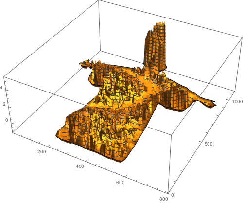
Here is a plot of the initial concentration for the diffusion equation within the Alma Mater.
Plot3D[Evaluate[H3[{x, y}]], {x, y} ? em, PlotRange -> All,
 MeshFunctions -> {#3 &}, PlotPoints -> 80, ImageSize -> 500]
Deciding on the Boundary Conditions
To solve the diffusion equation, we also need boundary conditions of the domain (at the boundary of the Alma Mater). To decide between Dirichlet and Neumann conditions, we solve a simple 1D model. The two gray lines show the path of the two points at the edge of the initial concentration bump.
Manipulate[
 Module[{nds, U, V},
  nds =
   NDSolveValue[{If[method == "Neumann",
      D[U[t, x], t] - D[U[t, x], {x, 2}] == NeumannValue[v, True],
      Sequence @@ {D[U[t, x], t] - D[U[t, x], {x, 2}] == 0,
        DirichletCondition[U[t, x] == v, True]}],

     U[0, x] == If[Abs[x] < Pi/2, H  Cos[x]^2, 1]},
                                 U , {x, -Pi, Pi}, {t, 0, 5},
    Method -> {"PDEDiscretization" -> {"MethodOfLines",

        "SpatialDiscretization" -> { "FiniteElement",

          "MeshOptions" -> {"MaxCellMeasure" -> 0.01}}}}];
  V  = Function[{t, x}, Evaluate[D[nds[t, x], x]/nds[t, x]]];
  With[{nds1 = nds, V1 = V},
   Manipulate[
    Module[{nds2R, nds2L},
     Column[{Plot[nds1[?, ?], {?, -Pi, Pi},
        AxesLabel -> {Style["x", Italic], Style["u", Italic]},

        PlotLabel -> Row[{Style["t", Italic], "=", ?}]],
       Plot3D[nds1[s, ?], {?, -Pi, Pi}, {s, 0, ?},
        MeshFunctions -> {#3 &},
        AxesLabel -> {Style["x", Italic], Style["t", Italic],
          Style["u", Italic]} ],

       nds2R = NDSolveValue[{X'[s] == V1[s, X[s]], X[0] == +Pi/2},
         X, {s, 0, ?}];

       nds2L = NDSolveValue[{X'[s] == V1[s, X[s]], X[0] == -Pi/2},
         X, {s, 0, ?}];

       ParametricPlot[
        Evaluate[{{nds2L[s], s}, {nds2R[s], s}}], {s, 0, ?},

        AxesLabel -> {Style["x", Italic], Style["t", Italic]},

        PlotStyle -> Gray,

        AspectRatio -> 1/GoldenRatio, PlotRange -> {{-Pi, Pi}, All}]
            }]],
    {{?, 1}, 0, 5, Appearance -> "Labeled"},
    TrackedSymbols :> {?}]]],
 {{method, "Neumann"}, {"Neumann", "Dirichlet"}},
 {{v, 1, "boundary condition value"} , -3, 3, Appearance -> "Labeled"},
 {{H, 2, "initial bump height"}, -3, 3, Appearance -> "Labeled"},
 TrackedSymbols :> {method, v, H}, SaveDefinitions -> True]
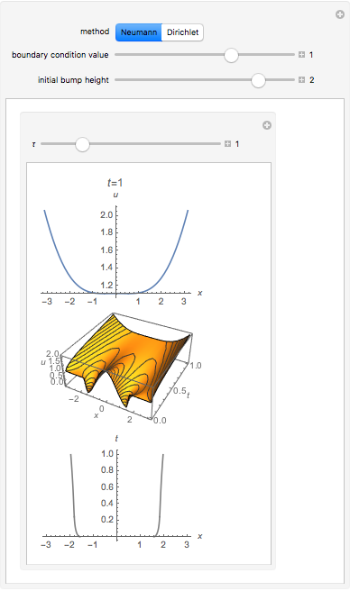
After some playing around one sees that Neumann boundary conditions with positive values seem to be a good choice to spread out the concentration out up to the outer boundary.
Solve the Diffusion Equation with Neumann Boundary Conditions
Now we solve the diffusion equation numerically. An appropriate value for the diffusion coefficient Subscript[c, D] and corresponding total integration time t can be found after some experimentation or some crude estimation based on the classic formula $?|{x,y}|^2??4c_Dt.$
cD = 50;
uSolN = NDSolveValue[{D[n[t, x, y], t] - cD Laplacian[n[t, x, y], {x, y}] ==
     NeumannValue[1, True],
     n[0, x, y] == 1 + H3[{x, y}]},
   n, {x, y} ? em, {t, 0, 100}, PrecisionGoal -> 5] // Quiet

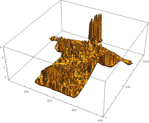
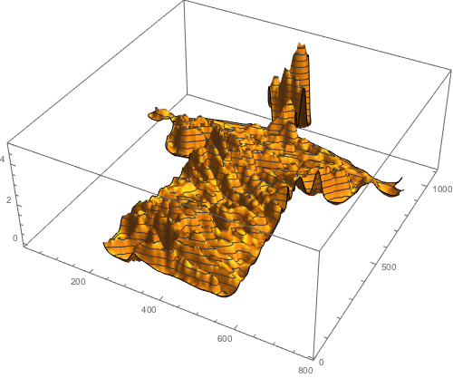
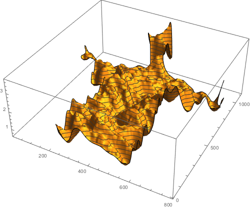
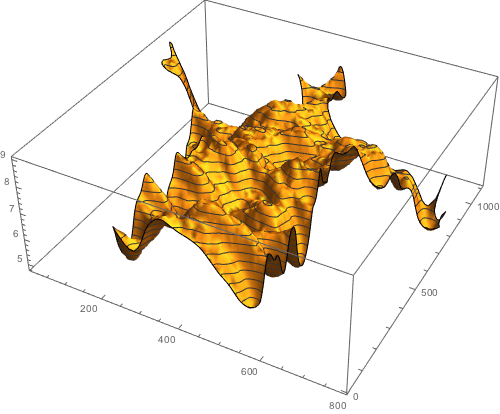
Here are a few plots of the concentration at various times (we show the concentration for t=0.01, t=0.5, t=5, and t=50). With increasing time the concentration differences even out. And the character shapes slowly disappear.
concentrationPlot[t_] :=
 Plot3D[Evaluate[uSolN[t, x, y]], {x, y} \[Element] em, PlotRange -> All,
  MeshFunctions -> {#3 &}, PlotPoints -> 80, ImageSize -> 500]

concentrationPlot[0.01]
concentrationPlot[0.5]
concentrationPlot[5]
concentrationPlot[50]
Calculate the Flow Field
But we are not interested in the concentration itself, but rather in the integrals of the flow of the concentration.
The flow vector field can be easily obtained by differentiating the interpolating function that represents the diffusion equation solution with respect to the coordinates.
vX[t_, x_Real, y_Real] = -D[uSolN[t, x, y], x]/uSolN[t, x, y]

vY[t_, x_Real, y_Real] = -D[uSolN[t, x, y], y]/uSolN[t, x, y]

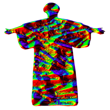
Here is a plot of the direction of the flow at t=0.1 and at the much later time t=10. Each color represent a flow direction.
colF = If[# == 10, White,
    ColorData["VisibleSpectrum"][380 + 370 (#1 + Pi)/(2 Pi)]] &;

vectorGrid[T_] := With[{t = T, pp = 800},
   Monitor[
    Table[If[srd[{x, y}] >= 0, 10,
      ArcTan[vX[t, 1. x, 1. y], vY[t, 1. x, 1. y]]],
                 {y, 0, 1100, 1100/pp}, {x, 0, 800, 800/pp}],
    N[y]]] /. Indeterminate -> 0.

ReliefPlot[vectorGrid[0.1], ColorFunction -> colF,
 ColorFunctionScaling -> False, AspectRatio -> Automatic, Frame -> False]
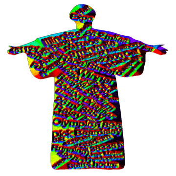
ReliefPlot[vectorGrid[10], ColorFunction -> colF,
 ColorFunctionScaling -> False, AspectRatio -> Automatic, Frame -> False]
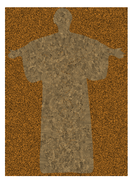
Here is a line integral convolution plot that shows the flow at some early time.
vectors =
  With[{t = 0.1, pp = 600},
   Monitor[
    Table[If[
      srd[{x, y}] > 0, {0, 0}, {vX[t, 1. x, 1. y], vY[t, 1. x, 1. y]}],
                 {y, 0, 1100, 1100/pp}, {x, 0, 800, 800/pp}],
    N[y]]];

ListLineIntegralConvolutionPlot[Map[Normalize, Transpose@vectors, {2}],
 PerformanceGoal -> "Quality",
 RasterSize -> 600, LineIntegralConvolutionScale -> 20,
 AspectRatio -> 11/8, Frame -> False]
Diffuse the Characters of the Words
For a few characters (M=20), we calculate their time evolution under the diffusion. To be time-efficient, we only diffuse/propagate the boundary points, rather than all interior points. The above-defined function makeFilledCurve will then reconstruct the full character. We use the "StiffnessSwitching" option for calculating along the flow lines to avoid getting stuck at potential abrupt function value changes.
M = 20;
Monitor[
  ptsA =
   Table[pts = MeshPrimitives[RegionBoundary[chars[[m]]], {0}];
                 ? = Length[pts];
    Table[NDSolveValue[{x'[t] == cD vX[t, x[t], y[t]],

       y'[t] == cD vY[t, x[t], y[t]],
                                              x[0] == pts[[j, 1, 1]],
       y[0] == pts[[j, 1, 2]]},
                                                {x[t], y[t]},  {t, 0,
       80},
                     PrecisionGoal -> 3, StartingStepSize -> 10^-4,
                    MaxSteps -> 10000,
      Method -> "StiffnessSwitching"] ,
                {j, ?}],
    {m, M}],
  {m, {j, ?}}];
Some examples of the propagated/diffused boundaries of the characters. The points of the boundaries are connected by line segments. To obtain smoother-looking curves, we will use splines in the final graphics. Early times are blue and later times are more red-like. The expansion of the characters is clearly visible.
Table[Show[Table[MeshRegion[ptsA[[k]] /. t -> 10^?,
        Style[MeshCells[RegionBoundary[chars[[k]]], 1],
     ColorData["ThermometerColors"][(? + 3)/5]]],
     {?, -3, 1, 0.1}], ImageSize -> 140], {k, 9}]
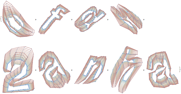
The following Manipulate allows to change the time, and so the character shape, interactively.
Manipulate[
 Show[Table[
    MeshRegion[ptsA[[m]] /. t -> ?,
     MeshCells[RegionBoundary[chars[[m]]], 1]], {m, M}],
   PlotRange -> {{100, 800}, {100, 1000}}, ImageSize -> 400] //
  Quiet, {?, 0, 50}]
Make the Dense Word Cloud(s)
Now we have all ingredients together to make a dense word cloud. We define a function that diffuses/propagates a point forward in time.
diffusionMove[{x0_, y0_}, T_] := #[T] & /@

  NDSolveValue[{x'[t] == cD vX[t, x[t], y[t]],
                                y'[t] == cD vY[t, x[t], y[t]],
                                x[0] == x0, y[0] == y0},
                    {x, y},  {t, T, T}, MaxStepSize -> 0.1,
                  PrecisionGoal -> 3, StartingStepSize -> 10^-4,
                 MaxSteps -> 500000, Method -> "StiffnessSwitching"]

outline = makeClosedCurve[RegionBoundary[mr], Identity];

rnA = RegionNearest[RegionBoundary@mr];
fix[{x_, y_}] := If[srd[{x, y}] <= 0, {x, y}, rnA[{x, y}]]
fix[Line[l_]] := Line[fix /@ l]
The function makeFlowImage generates a word cloud of the diffused-out characters at time t.
makeFlowImage[T_] :=
 Module[{mfc},
  Monitor[
   allCharsD =
     Table[Check[mfc = makeFilledCurve[chars[[k]], diffusionMove[#, T] &,
                        {RGBColor @@ charColors[[k, 1]], LightBlue}],

       mfc /. l_Line :> fix[l]],   {k, Length[chars]}];,
   Text@Row[{"Calculating diffusion shape for character ", k, " from ",
      Length[chars], " characters."}]];
  Graphics[{LightBlue, FilledCurve[outline], Black, outline, allCharsD},
   ImageSize -> 600]];
Looping over all boundary points of all characters shows how the characters spread out over time and fill the void to the Alma Mater boundary and between the characters and words.
Here are the outlines of the characters at various times.
makeFlowImage[0.5]
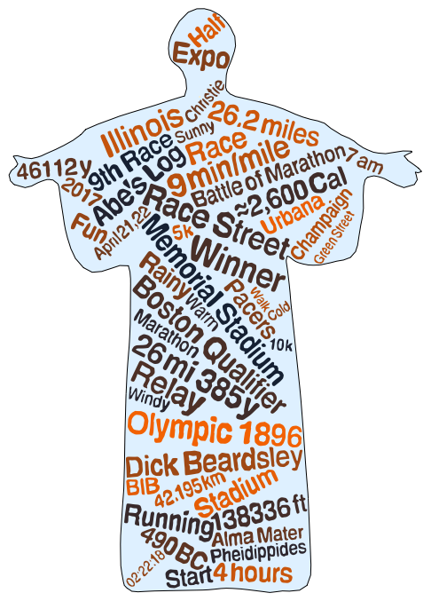
makeFlowImage[1]
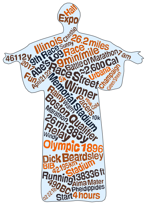
makeFlowImage[5]

makeFlowImage[10]

makeFlowImage[20]
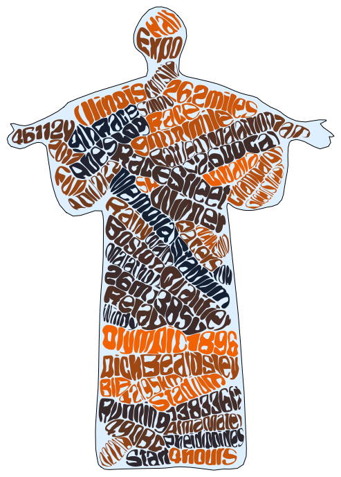
makeFlowImage[50]
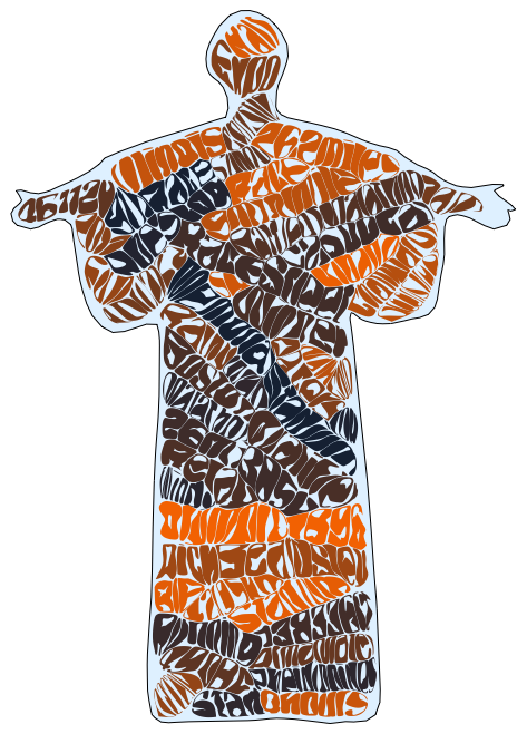
makeFlowImage[100]
 Attachments: